Tune Regression Model Using Experiment Manager
This example shows how to use Experiment Manager to optimize a machine learning
regression model. The goal is to create a regression model for the
carbig data set that has minimal cross-validation loss. Begin by
using the Regression Learner app to train all available regression models on the
training data. Then, improve the best model by exporting it to Experiment
Manager.
In Experiment Manager, use the default settings to minimize the cross-validation loss (that is, minimize the cross-validation root mean squared error). Investigate options that help improve the loss, and perform more detailed experiments. For example, fix some hyperparameters at their best values, add useful hyperparameters to the model tuning process, adjust hyperparameter search ranges, adjust the training data, and customize the visualizations. The final result is a model with better test set performance.
For more information on when to export models from Regression Learner to Experiment Manager, see Export Model from Regression Learner to Experiment Manager.
Load and Partition Data
In the MATLAB® Command Window, load the
carbigdata set, which contains measurements of cars made in the 1970s and early 1980s. Preprocess the data by categorizing the cars based on whether they were made in the USA, and remove rows where the table has missing values.load carbig Origin = categorical(cellstr(Origin)); Origin = mergecats(Origin,["France","Japan","Germany", ... "Sweden","Italy","England"],"NotUSA"); cars = table(Acceleration,Displacement,Horsepower, ... Model_Year,Origin,Weight,MPG); cars = rmmissing(cars)
Partition the data into two sets. Use approximately 80% of the observations for model training in Regression Learner, and reserve 20% of the observations for a final test set. Use
cvpartitionto partition the data.rng(0,"twister") % For reproducibility c = cvpartition(height(cars),"Holdout",0.2); trainingIndices = training(c); testIndices = test(c); carsTrain = cars(trainingIndices,:); carsTest = cars(testIndices,:);
Train Models in Regression Learner
If you have Parallel Computing Toolbox™, the Regression Learner app can train models in parallel. Training models in parallel is typically faster than training models in series. If you do not have Parallel Computing Toolbox, skip to the next step.
Before opening the app, start a parallel pool of process workers by using the
parpoolfunction.parpool("Processes")By starting a parallel pool of process workers rather than thread workers, you ensure that Experiment Manager can use the same parallel pool later.
Note
Parallel computations with a thread pool are not supported in Experiment Manager.
Open Regression Learner using the
carsTraintable and theMPGvariable as the response. Specify to use 3-fold cross-validation rather than the default 5-fold cross-validation, and set aside25percent of the imported data as a test set.regressionLearner(carsTrain,"MPG",KFold=3,TestDataFraction=0.25)To accept the options in the New Session from Arguments dialog box, click Start Session.
Visually inspect the predictors in the open Response Plot. In the X-axis section, select each predictor from the X list. Note that some of the predictors, such as
Displacement,Horsepower, andWeight, display similar trends.Before training models, use principal component analysis (PCA) to reduce the dimensionality of the predictor space. PCA linearly transforms the numeric predictors to remove redundant dimensions. On the Learn tab, in the Options section, click PCA.
In the Default PCA Options dialog box, click the check box to enable PCA. Select
Specify number of componentsas the component reduction criterion, and specify4as the number of numeric components. Click Save and Apply.To obtain the best model, train all preset models. On the Learn tab, in the Models section, click the arrow to open the gallery. In the Get Started group, click All. In the Train section, click Train All and select Train All. The app trains one of each preset model type, along with the default fine tree model, and displays the models in the Models pane.
To find the best result, sort the trained models based on the validation root mean squared error (RMSE). In the Models pane, open the Sort by list and select
RMSE
                            (Validation)
.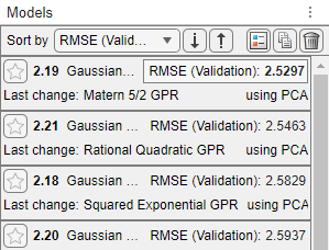
Note
Validation introduces some randomness into the results. Your model validation results can vary from the results shown in this example.
Assess Best Model Performance
For the model with the lowest RMSE, plot the predicted response versus the true response to see how well the regression model makes predictions for different response values. In this example, select the Matern 5/2 GPR model in the Models pane. On the Learn tab, in the Plots and Results section, click the arrow to open the gallery, and then click Predicted vs. Actual (Validation) in the Validation Results group.
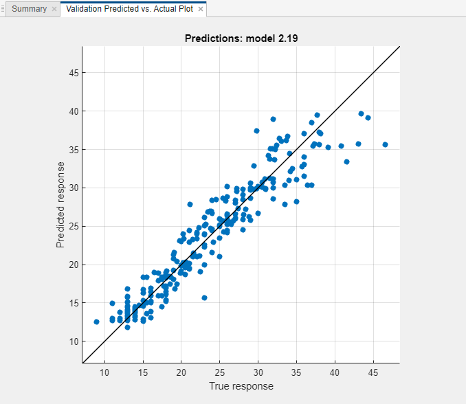
Overall, the GPR (Gaussian process regression) model performs well. Most predictions are near the diagonal line.
View the residuals plot. On the Learn tab, in the Plots and Results section, click the arrow to open the gallery, and then click Residuals (Validation) in the Validation Results group. The residuals plot displays the difference between the true and predicted responses.
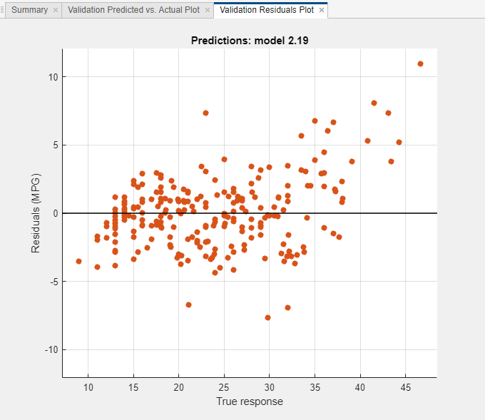
The residuals are scattered roughly symmetrically around 0.
Check the test set performance of the model. On the Test tab, in the Test section, click Test Selected. The app computes the test set performance of the model (which was trained on the training data set).
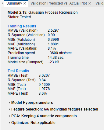
Compare the validation and test RMSE for the model. On the model Summary tab, compare the RMSE (Validation) value under Training Results to the RMSE (Test) value under Test Results. In this example, the validation RMSE overestimates the performance of the model on the test set.
Export Model to Experiment Manager
To try to improve the predictive performance of the model, export it to Experiment Manager. On the Learn tab, in the Export section, click Export Model and select Create Experiment. The Create Experiment dialog box opens.
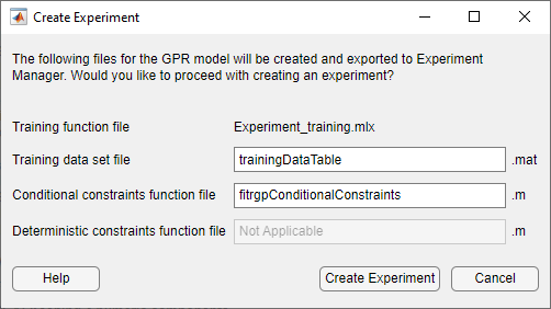
In the Create Experiment dialog box, click Create Experiment. The app opens Experiment Manager and a new dialog box.
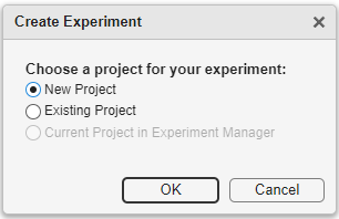
In the dialog box, choose a new or existing project for your experiment. For this example, create a new project, and specify
TrainGPRModelProjectas the filename in the Specify Project Folder Name dialog box.
Run Experiment with Default Hyperparameters
Run the experiment either sequentially or in parallel.
Note
If you have Parallel Computing Toolbox, save time by running the experiment in parallel. On the Experiment Manager tab, in the Execution section, select
Simultaneousfrom the Mode list.Otherwise, use the default Mode option of
Sequential.
On the Experiment Manager tab, in the Run section, click Run.
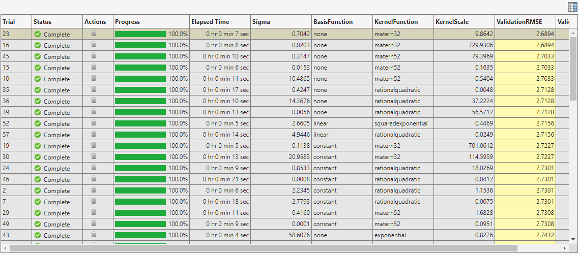
Experiment Manager opens a new tab that displays the results of the experiment. At each trial, the app trains a model with a different combination of hyperparameter values, as specified in the Hyperparameters table in the Experiment1 tab.
After the app runs the experiment, check the results. In the table of results, click the arrow for the ValidationRMSE column and select Sort in Ascending Order.
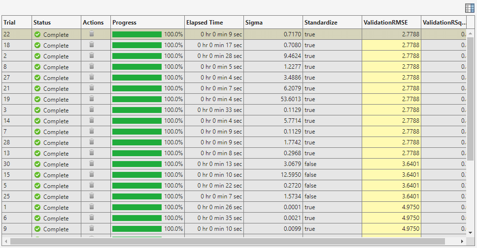
Notice that the app tunes the Sigma and Standardize hyperparameters by default.
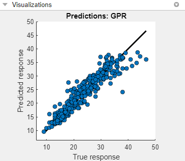
Check the predicted vs. actual plot for the model with the lowest RMSE. On the Experiment Manager tab, in the Review Results section, click Predicted vs. Actual (Validation). In the Visualizations pane, the app displays the plot for the model.
To better see the plot, drag the Visualizations pane below the Experiment Browser pane.

For this model, the predicted values are close to the true response values. However, the model tends to underestimate the true response for values between 40 and 50 miles per gallon.
Adjust Hyperparameters and Hyperparameter Values
Standardizing the numeric predictors before training seems best for this data set. To try to obtain a better model, specify the
Standardizehyperparameter value astrueand then rerun the experiment. Click the Experiment1 tab. In the Hyperparameters table, select the row for theStandardizehyperparameter. Then click Delete.In the Training Function section, click Edit to open the
Experiment1_training1.mlxfile.In the file, search for the lines of code that use the
fitrgpfunction. This function is used to create GPR models. Standardize the predictor data by using a name-value argument. In this case, adjust the four calls tofitrgpby adding'Standardize',trueas follows.regressionGP = fitrgp(predictors, response, ... paramNameValuePairs{:}, 'KernelParameters', kernelParameters, ... 'Standardize', true);
regressionGP = fitrgp(predictors, response, ...
    paramNameValuePairs{:}, 'Standardize', true);
regressionGP = fitrgp(trainingPredictors, trainingResponse, ...
    paramNameValuePairs{:}, 'KernelParameters', kernelParameters, ...
    'Standardize', true);
regressionGP = fitrgp(trainingPredictors, trainingResponse, ...
    paramNameValuePairs{:}, 'Standardize', true);
Save the code changes, and close the file.
On the Experiment Manager tab, in the Run section, click Run.
To further vary the models evaluated during the experiment, add hyperparameters to the model tuning process. On the Experiment1 tab, in the Hyperparameters section, click the arrow next to Add and select Add From Suggested List.
In the Add From Suggested List dialog box, select the
BasisFunction,KernelFunction, andKernelScalehyperparameters and click Add.Because the training data set includes a categorical predictor, the
pureQuadraticvalue must be deleted from the list of basis functions. In the Hyperparameters section, specify theBasisFunctionrange as["constant","none","linear"].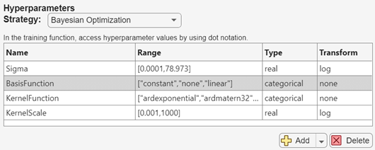
For more information on the hyperparameters you can tune for your model, see Export Model from Regression Learner to Experiment Manager.
For better results when tuning several hyperparameters, increase the number of trials. On the Experiment1 tab, in the Bayesian Optimization Options section, specify
60as the maximum number of trials.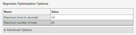
On the Experiment Manager tab, in the Run section, click Run.
Specify Training Data
Before running the experiment again, specify to use all the observations in
carsTrain. Because you reserved some observations for testing when you imported the training data into Regression Learner, all experiments so far have used only 75% of the observations in thecarsTraindata set.Save the
carsTraindata set as the filefullTrainingData.matin theTrainGPRModelProjectfolder, which contains the experiment files. To do so, right-click thecarsTrainvariable name in the MATLAB workspace, and click Save As. In the dialog box, specify the filename and location, and then click Save.On the Experiment1 tab, in the Training Function section, click Edit.
In the
Experiment1_training1.mlxfile, search for theloadcommand. Specify to use the fullcarsTraindata set for model training by adjusting the code as follows.% Load training data fileData = load("fullTrainingData.mat"); trainingData = fileData.carsTrain;
On the Experiment1 tab, in the Description section, change the number of observations to
314, which is the number of rows in thecarsTraintable.On the Experiment Manager tab, in the Run section, click Run.
Add Residuals Plot
You can add visualizations for Experiment Manager to return at each trial. In this case, specify to create a residuals plot. On the Experiment1 tab, in the Training Function section, click Edit.
In the
Experiment1_training1.mlxfile, search for theplotfunction. The surrounding code creates the validation predicted vs. actual plot for each trained model. Enter the following code to create a residuals plot. Ensure that the residuals plot code is within thetrainRegressionModelfunction definition.% Create validation residuals plot residuals = validationResponse - validationPredictions; f = figure("Name","Residuals (Validation)"); resAxes = axes(f); hold(resAxes,"on") plot(resAxes,validationResponse,residuals,"ko", ... "MarkerFaceColor","#D95319") yline(resAxes,0) xlabel(resAxes,"True response") ylabel(resAxes,"Residuals (MPG)") title(resAxes,"Predictions: GPR")
On the Experiment Manager tab, in the Run section, click Run.
In the table of results, click the arrow for the ValidationRMSE column and select Sort in Ascending Order.
Check the predicted vs. actual plot and the residuals plot for the model with the lowest RMSE. On the Experiment Manager tab, in the Review Results section, click Predicted vs. Actual (Validation). In the Visualizations pane, the app displays the plot for the model.
On the Experiment Manager tab, in the Review Results section, click Residuals (Validation). In the Visualizations pane, the app displays the plot for the model.
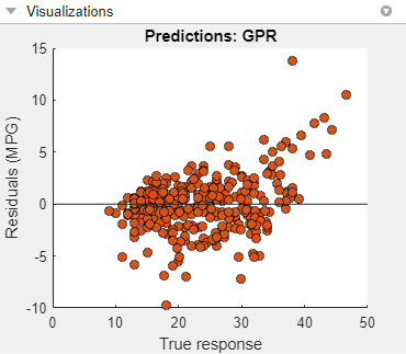
Both plots indicate that the model generally performs well.
Export and Use Final Model
You can export a model trained in Experiment Manager to the MATLAB workspace. Select the best-performing model from the most recently run experiment. On the Experiment Manager tab, in the Export section, click Export and select Training Output.
In the Export dialog box, change the workspace variable name to
finalGPRModeland click OK.The new variable appears in your workspace.
Use the exported
finalGPRModelstructure to make predictions using new data. You can use the structure in the same way that you use any trained model exported from the Regression Learner app. For more information, see Make Predictions for New Data Using Exported Model.In this case, predict the response values for the test data in
carsTest.testPredictedY = finalGPRModel.predictFcn(carsTest);
Compute the test RMSE using the predicted response values.
testRSME = sqrt((1/length(testPredictedY))* ...
    sum((carsTest.MPG - testPredictedY).^2))
testRSME = 2.6647The test RMSE is close to the validation RMSE computed in Experiment Manager (
2.6894). Also, the test RMSE for this tuned model is smaller than the test RMSE for the Matern 5/2 GPR model in Regression Learner (3.0267). However, keep in mind that the tuned model uses observations incarsTestas test data and the Regression Learner model uses a subset of the observations incarsTrainas test data.Create a predicted vs. actual plot and a residuals plot using the true test data response and the predicted response.
figure
line([min(carsTest.MPG) max(carsTest.MPG)], ...
    [min(carsTest.MPG) max(carsTest.MPG)], ...,
    "Color","black","LineWidth",2);
hold on
plot(carsTest.MPG,testPredictedY,"ko", ...
    "MarkerFaceColor","#0072BD");
hold off
xlabel("True response")
ylabel("Predicted response")
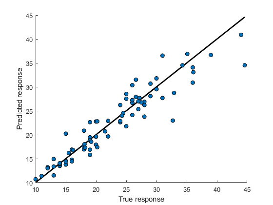
figure
residuals = carsTest.MPG - testPredictedY;
plot(carsTest.MPG,residuals,"ko", ...
    "MarkerFaceColor","#D95319")
hold on
yline(0)
hold off
xlabel("True response")
ylabel("Residuals (MPG)")

Both plots indicate that the model performs well on the test set.