Plan UAV Paths Using MATLAB Copilot

R2026b

Given a map of the environment, the next step is to determine how a UAV can move safely and efficiently from a starting location to a goal location. This requires solving a path planning problem, where the objective is to compute a collision-free path through the environment. This example uses the final occupancy map generated in the UAV Navigation in Unknown Environment with 2D Lidar SLAM example.

Prerequisites

Before completing this example, ensure you have:

• Set up MATLAB® Copilot and can access the MATLAB Copilot Chat interface as shown in MATLAB Copilot Basics (MATLAB Copilot).

• Familiarity with writing effective prompts to guide MATLAB Copilot. For more information, see Write Effective Prompts for MATLAB Copilot (MATLAB Copilot).

MATLAB Copilot does not necessarily return the same code in response to the same prompt. The code blocks in this example show typical examples of code that MATLAB Copilot generates. Review the code that is generated after you enter each prompt, before you paste it into MATLAB and run it.

Introduction to Path Planning Problem

A path planning problem involves determining how to move from a starting location to a goal location while avoiding obstacles in the environment.

To define a path planning problem, you must specify:

• State — The UAV position, represented as xy- coordinates

• Start state — The initial position of the UAV

• Goal state — The desired destination

• Constraints — Conditions such as obstacle avoidance and safety margins

The output of a path planning algorithm is a path, which is a sequence of waypoints that connects the start and goal while remaining in free space. A path describes where the UAV can go, but it does not specify how the UAV moves over time. Later in this example, you convert the path into a trajectory, which additionally defines position, velocity, and acceleration as functions of time.

Prepare Occupancy Map for Planning

Before computing a path, adjust the occupancy map to account for the UAV size, enabling it to maintain a safe distance from obstacles. You can do so by inflating the obstacles, which increases their size by a specified radius. Planning on the inflated map ensures that any path generated remains safely separated from obstacles.

Load the occupancy map data into the workspace.

load occMap.mat

Open the MATLAB Copilot Chat panel and enter this prompt:

I have loaded a 2-D occupancy map occMap for path planning. Prepare the occupancy map by inflating the obstacles with a safety radius of 1 m for the UAV, and 2 m for each obstacle. Then zoom the result so that the x axis range is [-85 10] and y axis range is [-15 80] in world coordinates.

This is a typical example of the code that MATLAB Copilot generates in response to this prompt. Review the code that is generated after you enter the prompt, before you paste it into MATLAB and run it.

% Combined inflation radius: UAV safety (1 m) + obstacle safety (2 m)
inflationRadius = 1 + 2;  % meters

% Create an independent copy of occMap
inflatedMap = copy(occMap);

% Inflate obstacles on the copy (radius in meters)
inflate(inflatedMap, inflationRadius);

% Display uninflated and inflated occupancy maps with specified world zoom
figure('Name','Uninflated and Inflated Occupancy Maps','NumberTitle','off','Color','w')

subplot(1,2,1)
show(occMap, 'world')
title('Uninflated Map')
axis equal
xlim([-85 10])
ylim([-15 80])

subplot(1,2,2)
show(inflatedMap, 'world')
title(sprintf('Inflated Map (radius = %.1f m)', inflationRadius))
axis equal
xlim([-85 10])
ylim([-15 80])

Plan Paths Using A* and RRT* Algorithms

Compute paths between a start and goal location using two different path planning algorithms:

• A* — A grid-based algorithm that searches for a short path on a discretized map.

• Rapidly-exploring random tree (RRT) — A sampling-based algorithm that explores the space randomly to find a feasible path.

Both planners use the same map, start point, and goal point, but can produce different paths.

Open the MATLAB Copilot Chat panel and enter this prompt:

Using the inflatedMap and start point [-75 0] and goal point [-5 20] meters in world coordinates, plan paths using A*. Measure planning time, compute path length. Store waypoints, planning time, and path length using variable names that end in AStar.

This is a typical example of the code that MATLAB Copilot generates in response to this prompt. Review the code that is generated after you enter the prompt, before you paste it into MATLAB and run it.

% Start and goal in world coordinates
startWorld = [-75 0];
goalWorld  = [-5  20];

% Create A* planner for the grid/world map
planner = plannerAStarGrid(inflatedMap);

% Plan and measure time
tic;
[pathAStar, debugInfo] = plan(planner, startWorld, goalWorld, 'world');
planningTimeAStar = toc;   % seconds

% pathAStar is n-by-2: [x y] in world coordinates when using 'world'
waypointsAStar = pathAStar;

% Compute Euclidean path length
diffs = diff(waypointsAStar, 1, 1);
segmentLengths = sqrt(sum(diffs.^2, 2));
pathLengthAStar = sum(segmentLengths);

Open the MATLAB Copilot Chat panel and enter this prompt:

Using the inflatedMap and start point [-75 0] and goal point [-5 20] meters in world coordinates, plan paths using RRT. Measure planning time, compute path length. Store waypoints, planning time, and path length using variable names that end in RRT.

This is a typical example of the code that MATLAB Copilot generates in response to this prompt. Review the code that is generated after you enter the prompt, before you paste it into MATLAB and run it.

% RRT planning between two world points using inflatedMap
startWorld = [-75 0];   % [x y]
goalWorld  = [-5 20];   % [x y]

% Create SE2 state space and validator tied to inflated occupancy map
ss = stateSpaceSE2;
sv = validatorOccupancyMap(ss);
sv.Map = inflatedMap;

% Small validation distance to check collisions along motion (meters)
sv.ValidationDistance = 0.01;

% Set state bounds from map world limits (x,y) and full yaw range
ss.StateBounds = [inflatedMap.XWorldLimits; inflatedMap.YWorldLimits; [-pi pi]];

% Create RRT planner. Increase MaxConnectionDistance if environment is sparse.
plannerRRTobj = plannerRRT(ss, sv, MaxConnectionDistance=1.0, MaxIterations=1e4, GoalBias=0.05);

% Define start and goal as SE2 states (x,y,theta). Use theta=0 for both.
startState = [startWorld 0];
goalState  = [goalWorld  0];

% For repeatable results (optional)
rng(0, 'twister');

% Plan and time it
tic;
[pthObj, solnInfoRRT] = plan(plannerRRTobj, startState, goalState);
planningTimeRRT = toc;

% Extract waypoints (2D positions) and compute path length
waypointsRRT = pthObj.States(:,1:2);
diffs = diff(waypointsRRT, 1, 1);
segmentLengths = sqrt(sum(diffs.^2, 2));
pathLengthRRT = sum(segmentLengths);

Compare Path Planning Results

Use MATLAB Copilot to generate code that visualizes both paths on the same map, compares planning time, and compares path length.

Open the MATLAB Copilot Chat panel and enter this prompt:

Plot the path generated by A Star and RRT planner. Compare the planning time and path length in a table.

This is a typical example of the code that MATLAB Copilot generates in response to this prompt. Review the code that is generated after you enter the prompt, before you paste it into MATLAB and run it.

% --- Plot A* and RRT paths on the inflated map ---
figure('Name','Planned Paths: A* vs RRT','NumberTitle','off','Color','w')
show(inflatedMap, 'world')
axis equal
xlim([-85 10])
ylim([-15 80])
hold on

% Plot start and goal
plot(startWorld(1), startWorld(2), 'gp', 'MarkerSize', 12, 'MarkerFaceColor','g') % start
plot(goalWorld(1),  goalWorld(2),  'rp', 'MarkerSize', 12, 'MarkerFaceColor','r') % goal

% Plot A* path
plot(waypointsAStar(:,1), waypointsAStar(:,2), '-b', 'LineWidth', 2)

% Plot RRT path
plot(waypointsRRT(:,1), waypointsRRT(:,2), '-m', 'LineWidth', 2)

legendEntries = {'Start','Goal','A* Path','RRT Path'};
legend(legendEntries,'Location','bestoutside')
title('A* (blue) and RRT (magenta) planned paths on inflated map')
hold off

% --- Create Comparison Table of Metrics ---
Planner = ["AStar"; "RRT"];
PlanningTime_s = [planningTimeAStar; planningTimeRRT];
PathLength_m    = [pathLengthAStar;   pathLengthRRT];
metricsTableAStarRRT = table(Planner, PlanningTime_s, PathLength_m);

% Display the table
disp(metricsTableAStarRRT)

    Planner    PlanningTime_s    PathLength_m
    _______    ______________    ____________

    "AStar"       0.10795           84.979   
    "RRT"         0.19335           102.69   

The A* planner produces a short and direct path because it systematically searches the grid to minimize path cost. In contrast, the RRT planner explores the environment through random sampling and might produce longer or less direct paths.

In this case:

• The A* path is shorter and more direct.

• The planning times are comparable, indicating that both planners solve this problem efficiently for this map size.

• The RRT path is less direct, and can vary between runs due to its probabilistic nature.

Although both planners complete in similar time, the higher path quality from A* makes it the preferred choice for this scenario. Based on these results, this example uses A* for the next step because it produces a more efficient and consistent path without increasing planning time.

Simulate UAV Motion Using the Planned Path

The A* planner returns a sequence of waypoints that define a collision‑free path in the environment. To simulate UAV motion, convert this path into a trajectory, which specifies how the UAV moves along the path over time.

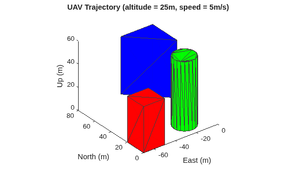
Use the same scenario geometry from the UAV Navigation in Unknown Environment with 2D Lidar SLAM example so that the UAV flies through a scene consistent with the environment used to generate the occupancy map. This results in a simulation scene that matches the earlier example.

Create the UAV scenario and add obstacles to match the reference environment:

scene = uavScenario(UpdateRate=10);
% Obstacle 1
addMesh(scene,"Polygon",{[-70 0; -50 0; -50 20; -70 20],[0 40]},[1 0 0]) 
% Obstacle 2
addMesh(scene,"cylinder",{[-20 15 10],[0 60]},[0 1 0])  
% Obstacle 3
addMesh(scene,"Polygon",{[0 50; 0 80; -30 80],[0 50]},[0 0 1]) 

Open the MATLAB Copilot Chat panel and enter this prompt:

Generate a UAV trajectory with an altitude of 25 meters and groundspeed of 5 m/s using the waypoints generated by A*. Simulate the trajectory in the UAV Scenario scene with a quadcopter.

This is a typical example of the code that MATLAB Copilot generates in response to this prompt. Review the code that is generated after you enter the prompt, before you paste it into MATLAB and run it.

% Desired altitude (positive up) and groundspeed
altitude = 25;    % meters above ground (positive)
groundSpeed = 5;  % m/s

% Convert ENU -> NED:
% - Swap East/North to become [North, East]
% - Use negative Z for altitude (Down is negative)
wptsENU = waypointsAStar;                % [x_east, y_north]
wptsNED_xy = wptsENU(:,[2,1]);           % [y_north, x_east] -> [X_North, Y_East]
wpts3D = [wptsNED_xy, -altitude*ones(size(wptsNED_xy,1),1)];  % N-by-3 [X Y Z(NED)]

% Compute cumulative distances in 3-D (or 2-D if you prefer) and TimeOfArrival
dists = [0; cumsum(sqrt(sum(diff(wpts3D,1,1).^2,2)))];   % meters
timeOfArrival = dists / groundSpeed;                     % seconds, same length as waypoints

% Create waypointTrajectory using TimeOfArrival
traj = waypointTrajectory(Waypoints = wpts3D, TimeOfArrival = timeOfArrival);

% Add a UAV platform to the scene using the trajectory
uavName = "Quadcopter";
uavPlat = uavPlatform(uavName, scene, Trajectory = traj);

% Add a quadrotor mesh to the platform for visualization

updateMesh(uavPlat, "quadrotor", {5}, [0 0 0], eul2tform([0 0 0]));

% Prepare for simulation and animate (safe loop)
setup(scene);

% Simulation end time from the trajectory (seconds)
simEndTime = traj.TimeOfArrival(end);

% Create 3-D view once
ax = show3D(scene);
axis(ax, 'equal');
view(3);
title(ax, sprintf('UAV Trajectory (altitude = %dm, speed = %dm/s)', altitude, groundSpeed));

% Initialize simulation time before the loop (place before while advance(scene))
simTime = 0;
dt = 1 / scene.UpdateRate;   % time step in seconds

% Run scenario but stop when simulation time passes the trajectory end time
while advance(scene)
    show3D(scene, "Parent", ax, "FastUpdate", true);
    drawnow limitrate

    % Increment tracked simulation time
    simTime = simTime + dt;

    % Break after we've simulated past the planned arrival time
    if simTime >= simEndTime
        break
    end
end

Next Steps

In this example, you used MATLAB Copilot to generate and compare path planning algorithms, select an appropriate planner, and simulate UAV motion using the resulting path.

To further explore path planning and UAV simulation, consider these additional tasks:

• Tune RRT parameters using MATLAB Copilot — Modify parameters such as MaxConnectionDistance, MaxIterations, and GoalBias to observe how they affect path quality and planning time. Use MATLAB Copilot to generate and test different configurations.

• Run multiple RRT trials — Since RRT is a probabilistic algorithm, run the planner multiple times with different random seeds, and compare the variability in path length and planning time.

• Modify safety margins — Change the inflation radius used in the occupancy map and observe how it affects the feasibility and shape of the planned paths.

• Extend to dynamic environments — Explore scenarios with moving obstacles using examples such as Simulate UAV Using Radar Sensor to Avoid Dynamic Obstacles.