Simulate GNSS Multipath Effects on UAV Flying in Urban Environment

This example shows how to simulate global navigation satellite system (GNSS), such as the Global Positioning System (GPS) receiver noise due to local obstructions in the environment of the receiver.

A GNSS receiver estimates its current position from the signals it obtains from satellites in view. When a receiver is in a location with many local obstructions, it can suffer from multipath. Multipath occurs when the signals from a satellite arrive at two or more paths. At most, one of these paths is a direct line-of-sight (LOS) from the satellite to the receiver. The remaining indirect paths are reflections from the local obstructions.

Each satellite signal contains a transmission timestamp that you can use with the receiver clock to compute the pseudorange between the satellite and the receiver. A satellite signal arriving on a indirect path results in an incorrect pseudorange that is larger than the pseudorange from a direct path. The incorrect pseudorange degrades the accuracy of the estimated receiver position.

This image shows a UAV flying over a street in a UAV scenario in New York City, with tall buildings on either side of the street. As the UAV flies, you can see a skyplot (Navigation Toolbox) on the right that shows the satellites in view of the receiver.

Create UAV Scenario with Buildings and Terrain

The scenario in this example contains an urban environment with tall buildings, centered in New York City.

Create a UAV scenario with the reference location set in New York City, and then add a terrain mesh using the GMTED2010 terrain model from the United States Geological Survey (USGS) and National Geospatial-Intelligence Agency (NGA). You must have an active internet connection to access this terrain data.

referenceLocation = [40.707088 -74.012146 0];
stopTime = 100;
scene = uavScenario(ReferenceLocation=referenceLocation,UpdateRate=10,StopTime=stopTime);
xTerrainLimits = [-200 200];
yTerrainLimits = [-200 200];

color = [0.6 0.6 0.6];
addMesh(scene,"terrain",{"gmted2010" xTerrainLimits yTerrainLimits},color)

Add building meshes from an OSM file of New York City, manhattan.osm. The OSM file was downloaded from https://www.openstreetmap.org, which provides access to crowdsourced map data from all over the world. The data is licensed under the Open Data Commons Open Database License (ODbL), https://opendatacommons.org/licenses/odbl/.

xBuildingLimits = [-150 150];
yBuildingLimits = [-150 150];
color = [0.6431 0.8706 0.6275];

addMesh(scene,"buildings",{"manhattan.osm" xBuildingLimits yBuildingLimits,"auto"},color)

Create a UAV platform that flies between the buildings, and add a GNSS measurement generator to the UAV platform.

uavTrajectory = waypointTrajectory([-100 -150 140; 60 120 140],TimeOfArrival=[0 stopTime],ReferenceFrame="ENU");

plat = uavPlatform("UAV",scene,Trajectory=uavTrajectory,ReferenceFrame="ENU");
updateMesh(plat,"quadrotor",{1},[1 0 0],eye(4));

gnss = uavSensor("GNSS",plat,gnssMeasurementGenerator(ReferenceLocation=referenceLocation));

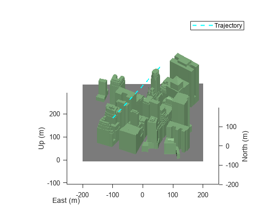
Visualize the scenario and the UAV trajectory.

fig = figure;
ax = show3D(scene);
uavPosition = uavTrajectory.lookupPose(linspace(0,stopTime,100));
hold on
uavTrajectoryLine = plot3(uavPosition(:,1),uavPosition(:,2),uavPosition(:,3),"--",LineWidth=1.5,Color="cyan");
legend(uavTrajectoryLine,"Trajectory",Location="northeast")

% Update axis plot settings for better readability.
helperUpdateScenarioView(ax)

Run Scenario and Visualize Multipath

Set up a top-down plot and sky plot to visualize the scenario by using show3D and skyplot (Navigation Toolbox), respectively.

The top-down plot represents the UAV platform as a blue dot, and shows the local obstructions that interfere with the GPS satellite signals.

The sky plot shows all of the GPS satellites that are currently in view of the UAV platform. Each satellite is in one of these categories, depending on its visibility from the UAV platform:

• Blocked — The GPS receiver detects no signal from the satellite.

• Multipath — The GPS receiver detects signals from the satellite, but with one or more reflections.

• Visible — The GPS receiver detects a signal, and has direct line-of-sight (LOS) with the satellite.

Note that the receiver can currently detect multiple signals from the same satellite.

Resize the figure to fit both plots.

clf(fig,"reset")
set(fig,Position=[400 458 1120 420])

Create a UI panel on the left side of the figure, and create axes for a top-view plot. Plot a marker to visualize the position of the UAV during simulation.

hScenePlot = uipanel(fig,Position=[0 0 0.5 1]);
ax = axes(hScenePlot);
[~, pltFrames] = show3D(scene,Parent=ax);
hold(ax,"on")
uavMarker = plot(pltFrames.UAV.BodyFrame,0,0,Marker="o",MarkerFaceColor="cyan");
uavTrajectoryLine = plot3(uavPosition(:,1),uavPosition(:,2),uavPosition(:,3),"--",LineWidth=1.5,Color="cyan");
legend(ax,[uavMarker uavTrajectoryLine],["UAV","Trajectory"],Location="northeast")
view(ax,[0 90])
axis(ax,"equal")
hold(ax,"off")

Create a UI panel on the right side of the figure, and create axes for a sky plot to show the satellite visibility. Add an empty sky plot to the panel. Set the color order to gray, red, and green representing blocked, multipath, and visible satellite statuses, respectively.

hSkyPlot = uipanel(fig,Position=[0.5 0 0.5 1]);
sp = skyplot(NaN,NaN,Parent=hSkyPlot);
title("GPS Satellites with LOS and Multipath Reception")
legend(sp)
colors = colororder(sp);
colororder(sp,[0.6*[1 1 1]; colors(7,:); colors(5,:)])

Set up and run the UAV scenario. At each step of the scenario:

1. Read the satellite pseudoranges.

2. Get the satellite azimuths and elevations from the satellite positions.

3. Categorize the satellites based on their status (Blocked, Multipath, or Visible).

4. Set different marker sizes so that you can see multiple measurements from the same satellite.

5. Update the sky plot.

currTime = gnss.SensorModel.InitialTime;
setup(scene)
while scene.IsRunning
    % Read the satellite pseudoranges.
    [~,~,p,satPos,status] = gnss.read();
    allSatPos = gnssconstellation(currTime);
    currTime = currTime + seconds(1/scene.UpdateRate);
    
    % Get the satellite azimuths and elevations from satellite positions.
    [~,trueRecPos] = plat.read;
    [az,el] = lookangles(trueRecPos,satPos,gnss.SensorModel.MaskAngle);
    [allAz,allEl,vis] = lookangles(trueRecPos,allSatPos,gnss.SensorModel.MaskAngle);
    allEl(allEl<0) = NaN;
    
    % Set categories of satellites based on the status (Blocked, Multipath, or Visible).
    groups = categorical([-ones(size(allAz)); status.LOS],[-1 0 1],["Blocked","Multipath","Visible"]); 
    
    % Set different marker sizes so that you can see the multiple measurements from the same satellite. 
    markerSizes = 100*ones(size(groups));
    markerSizes(groups=="Multipath") = 150;
    
    % Update the sky plot.
    set(sp,AzimuthData=[allAz; az],ElevationData=[allEl; el],GroupData=groups,MarkerSizeData=markerSizes);
    show3D(scene,Parent=ax,FastUpdate=true);
    drawnow

    % Advance the scene simulation time and update all sensor readings.
    advance(scene);
    updateSensors(scene)

end

Conclusion

This example has shown you how to generate raw GNSS measurements affected by multipath noise from local obstructions. You can use these measurements to estimate the position of the GPS receiver, or combine them with readings from other sensors, such as an inertial measurement unit (IMU), to improve the position estimation. For more information, see the Ground Vehicle Pose Estimation for Tightly Coupled IMU and GNSS (Navigation Toolbox).

Determining if a raw GNSS measurement contains multipath noise can be difficult, but you can use detection techniques such as innovation filtering, also known as residual filtering. For more information, see the Detect Multipath GPS Reading Errors Using Residual Filtering in Inertial Sensor Fusion (Navigation Toolbox) example.

Helper Functions

helperUpdateScenarioView updates scenario plot views for better readability.

function helperUpdateScenarioView(ax)
% Update the scenario view in axes handle AX.
meshes = findobj(ax,"type","patch");
for idx = 1:numel(meshes)
    meshes(idx).LineStyle = "none";
end
light(ax,"Position",[1 -5 6])
view(ax,[0 40])
end