Estimación de la pose del vehículo terrestre para IMU y GNSS estrechamente acoplados
Este ejemplo muestra cómo estimar la posición y orientación de un vehículo terrestre construyendo un filtro Kalman extendido estrechamente acoplado y usándolo para fusionar mediciones de sensores. Un filtro estrechamente acoplado fusiona lecturas de unidades de medición inercial (IMU) con lecturas sin procesar del sistema de navegación global por satélite (GNSS). Por el contrario, un filtro débilmente acoplado fusiona las lecturas de la IMU con las lecturas filtradas del receptor GNSS.
Diagrama de filtro ligeramente acoplado
Diagrama de filtro estrechamente acoplado
Aunque un filtro estrechamente acoplado requiere procesamiento adicional, puede usarlo cuando hay menos de cuatro señales de satélite GNSS disponibles o cuando algunas señales de satélite están dañadas por interferencias como el ruido de trayectorias múltiples. Este tipo de ruido puede ocurrir cuando un vehículo terrestre viaja a través de una parte de la carretera con muchas obstrucciones, como un cañón urbano, donde muchas superficies reflejan una combinación de señales hacia el receptor e interfieren con la señal directa. Debido a que el vehículo terrestre se encuentra en un entorno urbano con muchas posibilidades de que se produzca ruido de trayectorias múltiples, en este ejemplo se utiliza un filtro estrechamente acoplado.
Definir entrada de filtro
Especifique estos parámetros para la simulación del sensor:
Cantidades de movimiento de trayectoria
Tasa de muestreo de IMU
Frecuencia de muestreo del receptor GNSS
Archivo de mensajes de navegación RINEX
El archivo de mensajes de navegación RINEX contiene parámetros orbitales de satélites GNSS utilizados para calcular las posiciones y velocidades de los satélites. Las posiciones y velocidades de los satélites son importantes para generar los pseudodistancias y velocidades de pseudodistancia del GNSS.
load("routeNatickMATightlyCoupled","pos","orient","vel","acc","angvel","lla0","imuFs","gnssFs");
navfilename = "GODS00USA_R_20211750000_01D_GN.rnx";
Cree el objeto sensor IMU. Establezca los valores de desalineación de los ejes y de sesgo constante en 0 para simular la calibración.
imu = imuSensor(SampleRate=imuFs);
loadparams(imu,"generic.json","GenericLowCost9Axis");
imu.Accelerometer.AxesMisalignment = 100*eye(3);
imu.Accelerometer.ConstantBias = [0 0 0];
imu.Gyroscope.AxesMisalignment = 100*eye(3);
imu.Gyroscope.ConstantBias = [0 0 0];
Lea el archivo RINEX utilizando la función rinexread. Utilice solo el primer conjunto de satélites GPS del archivo y establezca el tiempo inicial para la simulación en el primer paso de tiempo del archivo.
data = rinexread(navfilename);
[~,idx] = unique(data.GPS.SatelliteID);
navmsg = data.GPS(idx,:);
t0 = navmsg.Time(1);
Cargue los parámetros de ruido, paramsTuned, para el sensor IMU y el receptor GNSS desde el archivo MAT tunedNoiseParameters.
load("tunedNoiseParameters.mat","paramsTuned");
accelNoise = paramsTuned.AccelerometerNoise;
gyroNoise = paramsTuned.GyroscopeNoise;
pseudorangeNoise = paramsTuned.exampleHelperINSGNSSNoise(1);
pseudorangeRateNoise = paramsTuned.exampleHelperINSGNSSNoise(2);
Configure la semilla RNG para producir resultados repetibles.
rng defaultCrear modelos de filtro y sensor de filtro
Para crear el filtro estrechamente acoplado utilizando el objeto insEKF, debe definir la conversión de los estados del filtro a mediciones GNSS sin procesar. Utilice la función auxiliar exampleHelperINSGNSS para definir esta conversión.
gnss = exampleHelperINSGNSS;
gnss.ReferenceLocation = lla0;
Defina un modelo IMU creando modelos de acelerómetro y giroscopio utilizando los objetos insAccelerometer y insGyroscope, respectivamente.
accel = insAccelerometer;
gyro = insGyroscope;
Cree el filtro utilizando el modelo del sensor IMU, el modelo del sensor GNSS sin procesar y un modelo de movimiento de pose 3D representado como un objeto insMotionPose.
filt = insEKF(accel,gyro,gnss,insMotionPose);
Establezca los estados iniciales del filtro utilizando los parámetros ajustados desde paramsTuned.
filt.State = paramsTuned.InitialState;
filt.StateCovariance = paramsTuned.InitialStateCovariance;
filt.AdditiveProcessNoise = paramsTuned.AdditiveProcessNoise;
Estimar la pose del vehículo
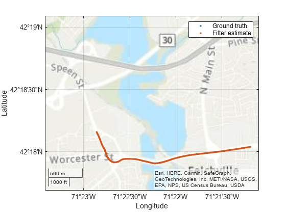
Cree una figura en la que ver la estimación de posición del vehículo terrestre durante el proceso de filtrado.
figure
posLLA = ned2lla(pos,lla0,"ellipsoid");
geoLine = geoplot(posLLA(1,1),posLLA(1,2),".",posLLA(1,1),posLLA(1,2),".");
geolimits([42.2948 42.3182],[-71.3901 -71.3519])
geobasemap topographic
legend("Ground truth","Filter estimate")
Asigne una matriz en la que almacenar los resultados de la estimación de posición.
numSamples = size(pos,1);
estPos = NaN(numSamples,3);
estOrient = ones(numSamples,1,"quaternion");
imuSamplesPerGNSS = imuFs/gnssFs;
numGNSSSamples = numSamples/imuSamplesPerGNSS;
Establezca el tiempo de simulación actual en el tiempo inicial especificado.
t = t0;
Fusione la IMU y las mediciones GNSS sin procesar. En cada iteración, fusione las mediciones del acelerómetro y giroscopio con las mediciones GNSS por separado para actualizar los estados del filtro, con las matrices de covarianza definidas por los parámetros de ruido cargados previamente. Después de actualizar el estado del filtro, registre los nuevos estados de posición y orientación. Finalmente, prediga los estados del filtro para el siguiente paso de tiempo.
for ii = 1:numGNSSSamples
    for jj = 1:imuSamplesPerGNSS
        imuIdx = (ii-1)*imuSamplesPerGNSS + jj;
        [accelMeas,gyroMeas] = imu(acc(imuIdx,:),angvel(imuIdx,:),orient(imuIdx,:));

        fuse(filt,accel,accelMeas,accelNoise);
        fuse(filt,gyro,gyroMeas,gyroNoise);

        estPos(imuIdx,:) = stateparts(filt,"Position");
        estOrient(imuIdx,:) = quaternion(stateparts(filt,"Orientation"));

        t = t + seconds(1/imuFs);
        predict(filt,1/imuFs);
    end
Actualice las posiciones de los satélites y las mediciones GNSS sin procesar.
    gnssIdx = ii*imuSamplesPerGNSS;
    recPos = posLLA(gnssIdx,:);
    recVel = vel(gnssIdx,:);
    [satPos,satVel,satIDs] = gnssconstellation(t,"RINEXData",navmsg);
    [az,el,vis] = lookangles(recPos,satPos);
    [p,pdot] = pseudoranges(recPos,satPos(vis,:),recVel,satVel(vis,:));
    z = [p; pdot];
Actualizar las posiciones de los satélites en el modelo GNSS.
    gnss.SatellitePosition = satPos(vis,:);
    gnss.SatelliteVelocity = satVel(vis,:);
Fusione las mediciones GNSS sin procesar.
    fuse(filt,gnss,z, ...
        [pseudorangeNoise*ones(1,numel(p)),pseudorangeRateNoise*ones(1,numel(pdot))]);
    estPos(gnssIdx,:) = stateparts(filt,"Position");
    estOrient(gnssIdx,:) = quaternion(stateparts(filt,"Orientation"));
Actualice el gráfico de estimación de posición.
    estPosLLA = ned2lla(estPos,lla0,"ellipsoid");
    set(geoLine(1),LatitudeData=posLLA(1:gnssIdx,1),LongitudeData=posLLA(1:gnssIdx,2));
    set(geoLine(2),LatitudeData=estPosLLA(1:gnssIdx,1),LongitudeData=estPosLLA(1:gnssIdx,2));
    drawnow limitrate
end
Validar resultados
Calcule el error RMS para validar los resultados. El filtro estrechamente acoplado utiliza las lecturas del sensor proporcionadas para estimar la pose del vehículo terrestre con un error RMS relativamente bajo.
posDiff = estPos - pos;
posRMS = sqrt(mean(posDiff.^2));
disp(['3-D Position RMS Error — X: ',num2str(posRMS(1)),', Y:', ...
    num2str(posRMS(2)),', Z: ',num2str(posRMS(3)),' (m)'])
3-D Position RMS Error - X: 0.8522, Y:0.62864, Z: 0.9633 (m)
orientDiff = rad2deg(dist(estOrient,orient));
orientRMS = sqrt(mean(orientDiff.^2));
disp(['Orientation RMS Error — ',num2str(orientRMS),' (degrees)'])
Orientation RMS Error - 4.0385 (degrees)