Multiplexing and Demultiplexing of CAN Messages

R2026b

Introduction

This example shows how to apply multiplexing and demultiplexing to CAN messages.

Multiplexing is a method used in CAN bus communication to increase the number of transmitted signals, at the cost of reducing the effective sample rate of each signal.

Multiplexed signals belong to the same CAN frame, but may have overlapping bit layouts. The interpretation of the bit pattern is conditional, and it depends on the value of another signal, called multiplexor.

Consider, as an example, the following sequence of a multiplexed OBD-II (On-Board Diagnostics) frame, as retrieved using the CAN Explorer app:

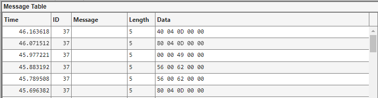
The interpretation of the first two data bytes depends on the value of the third byte, which corresponds to the OBD-II PID.

Specifically, the frame carries three different signals, with overlapping bit layout, as shown in the following figures.

Engine Torque, OBD-II PID = 98 (dec), 62 (hex)

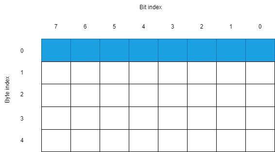
Accelerator Pedal Position, OBD-II PID = 73 (dec), 49 (hex)

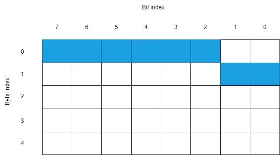
Vehicle Speed, OBD-II PID = 13 (dec), 0D (hex)

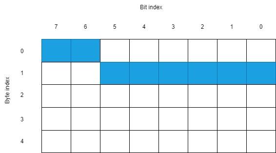
Multiplexor Signal

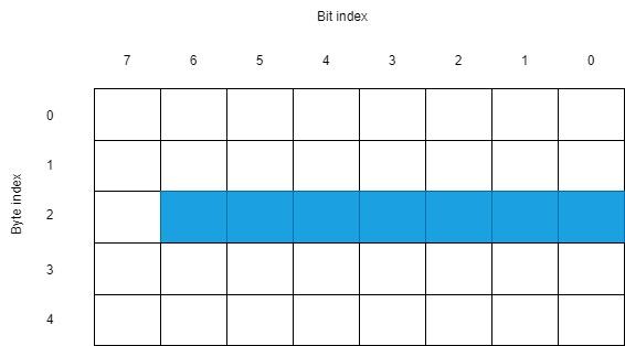
Note that the multiplexor signal has a bit layout that does not overlap with the other three signals.

In the following sections, actual recorded signals will be multiplexed and transmitted using a Simulink® model.

The CAN frames are then received in the CAN Explorer App, and eventually demultiplexed with a few lines of MATLAB® code.

Multiplexing and Transmission in Simulink

Recorded signals for the actual engine percent torque, the accelerator pedal position and the vehicle speed are available in a MAT file, in the form of timeseries. Data has been recorded from 0 to 25 seconds.

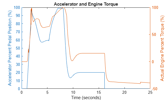
load("Logged_OBD2_Data.mat");

It is interesting to inspect the recorded signals; in particular, as shown in the following, the engine torque is negative when the accelerator position goes to 0. This is a common situation known as engine braking, and indeed the vehicle speed decreases accordingly.

figure;
yyaxis("left");
plot(Accelerator);
yyaxis("right");
plot(Engine_Torque);
title("Accelerator and Engine Torque");

figure
plot(Vehicle_Speed);
title("Vehicle Speed");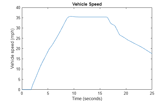

This data is input to the following Simulink model via From Workspace blocks.

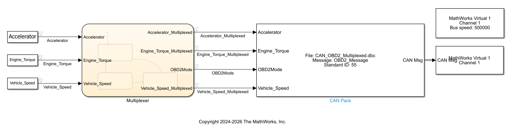
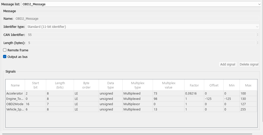
The CAN Pack block is configured as follows, based on the DBC file CAN_OBD2_Multiplexed.dbc. The file contains the definition of a single multiplexed CAN frame, with one multiplexor named OBD2Mode.

The input signals are fed into a Multiplexer block, which is implemented with a Stateflow® Chart. This is a particularly convenient approach for time-based multiplexing.

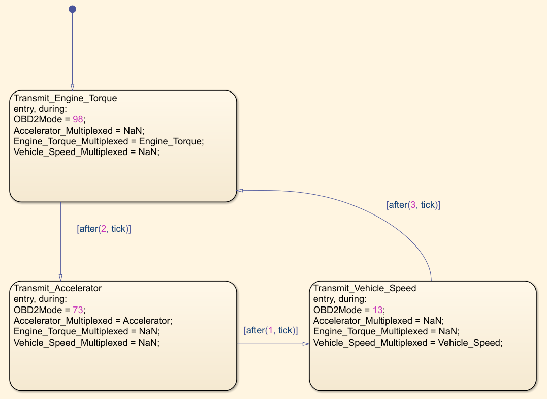
This state machine encompasses three mutually exclusive states. When the state Transmit_Engine_Torque is active, the engine torque signal as well as its corresponding OBD-II PID are transmitted, while the two other signals are set to NaN, because their values are missing. A similar logic applies to the two other states, namely, Transmit_Accelerator and Transmit_Vehicle_Speed.

Switching between states follows a time-based logic: the Transmit_Engine_Torque is active for two simulation time steps, the Transmit_Accelerator state for 1 time step, and the Transmit_Vehicle_Speed state is active for 3 time steps, before transitioning back to the first state. The tick keyword in Stateflow refers to an activation of the diagram at each time step, as triggered by the Simulink solver.

The following parameters are used to control the simulation of the Simulink model. Simulation pacing, to achieve near wall-clock time execution, is enabled.

Ts = 0.1; % [s]
StartTime = 0; % [s]
StopTime = 25; % [s]

After running the simulation, it is interesting to inspect the multiplexed signals, as well as the multiplexor.

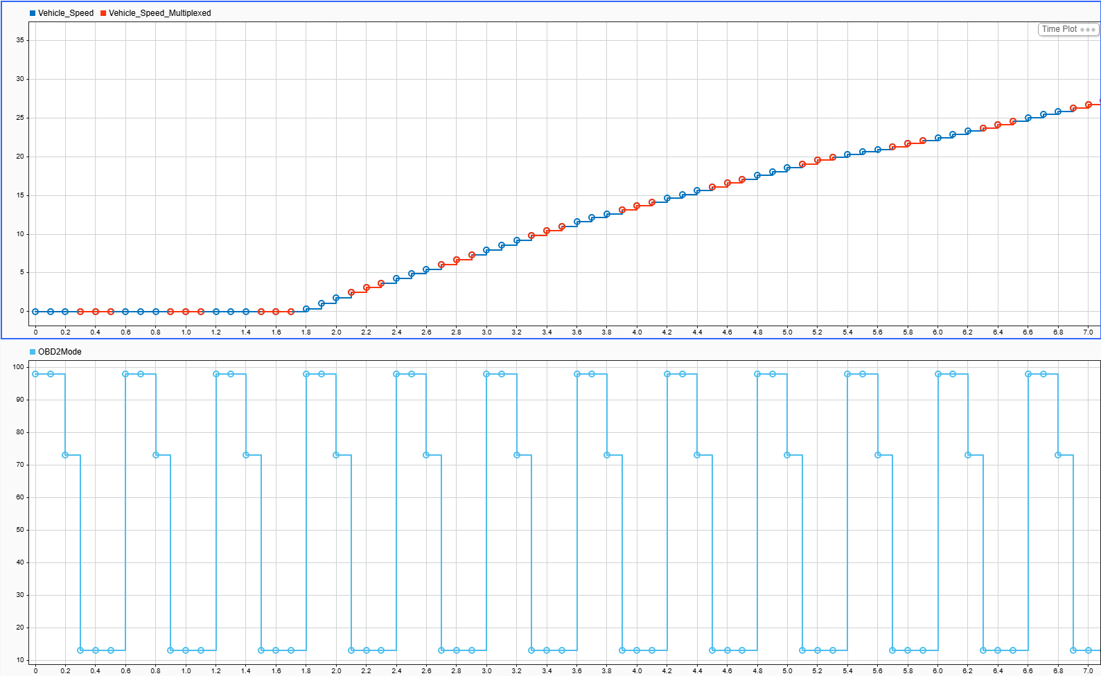
The multiplexor periodically switches between the values of 98, 73 and 13, corresponding to the OBD-II PIDs of the three signals. In particular, when the multiplexor value is 13, the associated Vehicle Speed signal is active; otherwise, that signal is not available.

This graph conveys the notion that multiplexing effectively introduces a downsampling of the original time series, as shown by the comparison between the original and multiplexed Vehicle Speed signal.

Reception and Demultiplexing in MATLAB

Open and configure the CAN Explorer App to receive the messages on the MathWorks Virtual Channel 1. Then, run the Simulink model to receive the messages, and export them to a MATLAB workspace variable. In this example, the variable is called canExplorerMsgs, and it is available in the canExplorerMsgs.mat file.

Create a CAN database object for the file CAN_OBD2_Multiplexed.dbc. Decode the messages using the database object and the canMessageTimetable and canSignalTimetable functions.

load("canExplorerMsgs.mat");
db = canDatabase("CAN_OBD2_Multiplexed.dbc");
msgsTT = canMessageTimetable(canExplorerMsgs, db);
sigsTT = canSignalTimetable(msgsTT)

sigsTT = 251×4 timetable
       Time       Vehicle_Speed    Accelerator    OBD2Mode    Engine_Torque
    __________    _____________    ___________    ________    _____________

    12.557 sec         NaN              NaN          98              0     
    12.657 sec         NaN              NaN          98              0     
    12.882 sec         NaN                0          73            NaN     
    12.976 sec           0              NaN          13            NaN     
    13.07 sec            0              NaN          13            NaN     
    13.281 sec           0              NaN          13            NaN     
    13.797 sec         NaN              NaN          98              0     
    13.967 sec         NaN              NaN          98              0     
    14.057 sec         NaN                0          73            NaN     
    14.147 sec           0              NaN          13            NaN     
    14.237 sec           0              NaN          13            NaN     
    14.327 sec           0              NaN          13            NaN     
    14.417 sec         NaN              NaN          98              7     
    14.507 sec         NaN              NaN          98             23     
    14.597 sec         NaN           39.608          73            NaN     
    14.687 sec           0              NaN          13            NaN     


      ⋮

If any CAN messages use multiplexing, these functions automatically apply demultiplexing. For a given message, the signals in the sigsTT timetable are assigned a value of NaN when they are not demultiplexed by the multiplexor value carried in that message.

Demultiplexed signals can be used as regular signals in data analysis and visualization. Data analysis functions, such as mean, provide arguments to control whether missing values should be included in calculations. In addition, visualization functions simply do not display missing data, as shown in the figure below.

vAverage = mean(sigsTT.Vehicle_Speed, "omitnan")

vAverage = 
24.5360

figure
plot(sigsTT.Time, sigsTT.Vehicle_Speed)
title("Vehicle Speed - Demultiplexed");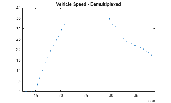

The figure clearly shows that demultiplexed signals are effectively downsampled. Moreover, the initial time is different from that of the simulation, due to the delay introduced by the user between starting the CAN Explorer App and starting the Simulink simulation. The time range of about 25 seconds is, however, coherent with the simulation time range, due to simulation pacing.