mlpt
Multiscale local 1-D polynomial transform
Syntax
Description
[ returns
the multiscale local polynomial 1-D transform (MLPT) of input signal coefs,T,coefsPerLevel,scalingMoments]
= mlpt(x,t)x sampled
at the sampling instants, t. If x or t contain NaNs,
the union of the NaNs in x and t is
removed before obtaining the mlpt.
[ returns
the transform for coefs,T,coefsPerLevel,scalingMoments]
= mlpt(x,t,numLevel)numLevel resolution levels.
[ uses uniform sampling instants
for coefs,T,coefsPerLevel,scalingMoments]
= mlpt(x)x as the time instants if x does
not contain NaNs. If x contains NaNs,
the NaNs are removed from x and
the nonuniform sampling instants are obtained from the numeric elements
of x.
[ specifies
coefs,T,coefsPerLevel,scalingMoments]
= mlpt(___,Name=Value)mlpt properties using one or more name-value arguments and
any of the previous syntaxes. For example, mlpt(x,DualMoments=4)
specifies four dual vanishing moments.
Examples
Create a signal with nonuniform sampling and verify good reconstruction.
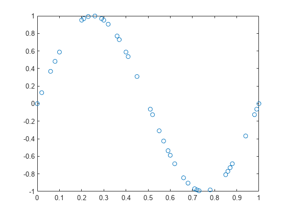
Create and plot a sine wave with nonuniform sampling.
timeVector = 0:0.01:1;
sineWave = sin(2*pi*timeVector);

samplesToErase = randi(100,1,100);
sineWave(samplesToErase) = [];
timeVector(samplesToErase) = [];

plot(timeVector,sineWave,"o")
grid on
title("Signal")
xlabel("Time (s)")
ylabel("Amplitude")
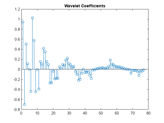
Use mlpt to obtain the multiscale local 1-D polynomial transform of the signal. Visualize the coefficients.
[coefs,T,coefsPerLevel,scalingMoments] = mlpt(sineWave,timeVector);
stem(coefs)
grid on
title("Wavelet Coefficients")
Use imlpt to obtain the inverse multiscale local 1-D polynomial transform of the coefficients. Plot the original signal and the reconstruction.
y = imlpt(coefs,T,coefsPerLevel,scalingMoments);

plot(timeVector,sineWave,"o")
hold on
plot(T,y,"x")
hold off
grid on
legend("Original Signal","Reconstruction")
xlabel("Time (s)")
ylabel("Amplitude")
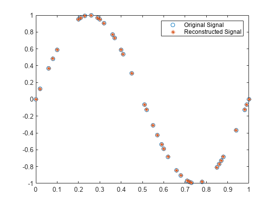
Inspect the total error to verify good reconstruction.
reconstructionError = sum(abs(y'-sineWave))
reconstructionError =
3.0396e-15
Specify nondefault dual moments by using the mlpt function. Compare the results of analysis and synthesis using the default and nondefault dual moments.
Create an input signal and visualize it.
t = linspace(0,1,200)';
x = cos(10*pi*t.^2);
plot(t,x)
title("Signal")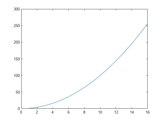
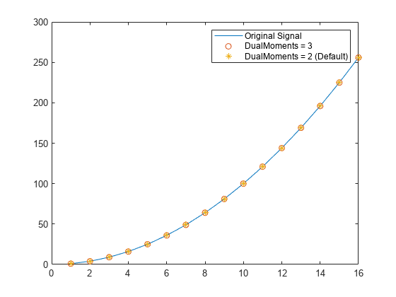
By default, DualMoments, the number of dual vanishing moments, is 2. Perform the forward and inverse transform for the input signal twice, with DualMoments set to 2 and 3.
[w2,t2,nj2,scalingmoments2] = mlpt(x,t);
y2 = imlpt(w2,t2,nj2,scalingmoments2);

[w3,t3,nj3,scalingmoments3] = mlpt(x,t,DualMoments=3);
y3 = imlpt(w3,t3,nj3,scalingmoments3,DualMoments=3);
Plot both reconstructions.
plot(t,x)
hold on
plot(t2,y2,'o')
plot(t3,y3,'*')
hold off
legend("Original", ...
       "DualMoments = 2", ...
       "DualMoments = 3");
For each reconstruction, compute the mean error. Verify perfect reconstruction.
fprintf("Mean Error\nDualMoments = 2: %e\nDualMoments = 3: %e", ...
    mean(abs(y2-x)),mean(abs(y3-x)))
Mean Error
DualMoments = 2: 1.539914e-16
DualMoments = 3: 7.797582e-17
Resolution levels are the number of cascaded local polynomial smoothing operations. The details at each resolution level are obtained by predicting one half the samples based on a local polynomial interpolation of the other half. The difference between the predicted and actual values are the details at each resolution level. The scaling coefficients at each coarser resolution level are smoother versions of the higher resolution scaling coefficients. Only the final-level scaling coefficients are retained.
Increasing the number of resolution levels enables you to analyze narrowband coefficients for a computational and memory cost.
Create a dual-tone input signal, x, that contains high and low frequencies.
fs = 1000;
t = (0:1/fs:10)';
x = sin(499*pi.*t) + sin(2*pi.*t);
Use mlpt to obtain coefficients for minimum and maximum resolution levels. Print the computation time.
tic
[w1,~,nj1,m1] = mlpt(x,t,1);
computationTime1 = toc;
disp("Level one computation time: "+computationTime1+" seconds")
Level one computation time: 0.83236 seconds
tic
[w13,~,nj13,m13] = mlpt(x,t,13);
computationTime13 = toc;
disp("Level thirteen computation time: "+computationTime13+" seconds")
Level thirteen computation time: 1.2393 seconds
If your time instants are not known or specified, you can calculate the MLPT using default time instants.
Load a data signal corrupted with NaNs and with unknown time instants. Calculate the MLPT without specifying time instants. The resulting implied time instants is a vector of valid indices of the corrupted signal.
load CorruptedData

[w,t,nj,scalingMoments] = mlpt(yCorrupt);
Calculate the inverse MLPT and visualize the results. Reinsert NaNs to visualize gaps in the signal.
z = imlpt(w,t,nj,scalingMoments);

zToPlot = NaN(numel(yCorrupt),1);
zToPlot(t) = z;

plot(yCorrupt,LineWidth=2.5)
hold on
plot(zToPlot,LineWidth=1)
hold off
legend("Original Signal","Reconstructed Signal")
xlabel("Time Instants")

Input Arguments
Name-Value Arguments
Output Arguments
Algorithms
Maarten Jansen developed the theoretical foundation of the multiscale
local polynomial transform (MLPT) and algorithms for its efficient
computation [1][2][3]. The MLPT uses a lifting scheme, wherein a kernel
function smooths fine-scale coefficients with a given bandwidth to
obtain the coarser resolution coefficients. The mlpt function uses only local polynomial
interpolation, but the technique developed by Jansen is more general
and admits many other kernel types with adjustable bandwidths [2].
References
[1] Jansen, Maarten. “Multiscale Local Polynomial Smoothing in a Lifted Pyramid for Non-Equispaced Data.” IEEE Transactions on Signal Processing 61, no. 3 (February 2013): 545–55. https://doi.org/10.1109/TSP.2012.2225059.
[2] Jansen, Maarten, and Mohamed Amghar. “Multiscale Local Polynomial Decompositions Using Bandwidths as Scales.” Statistics and Computing 27, no. 5 (September 2017): 1383–99. https://doi.org/10.1007/s11222-016-9692-8.
[3] Jansen, Maarten, and Patrick Oonincx. Second Generation Wavelets and Applications. London ; New York: Springer, 2005.
Version History
Introduced in R2017a