Main Content

filterbank

Shearlet system filters

Description

psi = filterbank(sls) returns the Fourier transforms of the shearlet filters defined by the shearlet system sls as a 3-D real-valued array. The array size is M-by-N-by-K, where M and N are the values of the two-element row vector ImageSize of sls. K is the number of shearlets including the lowpass filter, K = numshears(sls) + 1.

example

[psi,scale] = filterbank(sls) returns the scale parameters of the shearlet filters as a K-by-1 integer vector. K is the number of shearlets including the lowpass filter, K = numshears(sls) + 1.

[psi,scale,shear] = filterbank(sls) returns the shearing parameters of the shearlet filters as a K-by-1 integer vector. K is the number of shearlets including the lowpass filter, K = numshears(sls) + 1.

[psi,scale,shear,cone] = filterbank(sls) returns the frequency cones of the shearlet filters as a K-by-1 cell array of characters. K is the number of shearlets including the lowpass filter, K = numshears(sls) + 1.

example

Examples

collapse all

Load an image. Create a shearlet system that can be used with the image.

load clown
sls = shearletSystem('ImageSize',size(X))
sls = 
  shearletSystem with properties:

         ImageSize: [200 320]
         NumScales: 4
    PreserveEnergy: 0
     TransformType: 'real'
    FilterBoundary: 'periodic'
         Precision: 'double'

Obtain the shearlet filters defined by the shearlet system.

psi = filterbank(sls);

Obtain the shearlet transform of the image.

cfs = sheart2(sls,X);

Confirm that the size of the third dimension of psi is equal to the size of the third dimension of cfs.

[size(psi,3) size(cfs,3)]
ans = 1×2

    41    41

Create a complex-valued shearlet system for 256-by-256 images with truncated boundaries and four scales.

sls = shearletSystem('TransformType','complex',...
    'ImageSize',[256 256],...
    'FilterBoundary','truncated',...
    'NumScales',4);

Obtain the shearlet filters and their geometric interpretations.

[psi,scale,shear,cone] = filterbank(sls);

Different scales can have a different number of shears. The scales in the shearlet system range from 0 to 3 inclusive. Find the range of shears per scale.

for k=0:3
    ind = find(scale==k);
    fprintf('scale: %d  shear range: [%d:%d]\n',...
        k,min(shear(ind)),max(shear(ind)))
end
scale: 0  shear range: [-1:1]
scale: 1  shear range: [-2:2]
scale: 2  shear range: [-2:2]
scale: 3  shear range: [-3:3]

Display the unique frequency cone labels.

unique(cone)
ans = 5x1 cell
    {'B'}
    {'L'}
    {'R'}
    {'T'}
    {'X'}

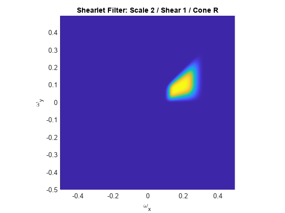
Find the shearlet filter at scale 2 with shear parameter equal to 1 and whose support is in the 'R' frequency cone.

vScale = 2;
vShear = 1;
vCone = 'R';
ind = (scale'==vScale)&(shear'==vShear)&([cone{:}]==vCone);
shFilter = psi(:,:,ind);

Plot the shearlet filter.

omegax = -1/2:1/256:1/2-1/256;
omegay = omegax;
surf(omegax,flip(omegay),shFilter,'EdgeColor','none')
view(0,90)
xlabel('\omega_x')
ylabel('\omega_y')
str = sprintf('Shearlet Filter: Scale %d / Shear %d / Cone %c',...
    vScale,vShear,vCone);
title(str)
axis equal
axis tight

Figure contains an axes object. The axes object with title Shearlet Filter: Scale 2 / Shear 1 / Cone R, xlabel omega indexOf x baseline, ylabel omega indexOf y baseline contains an object of type surface.

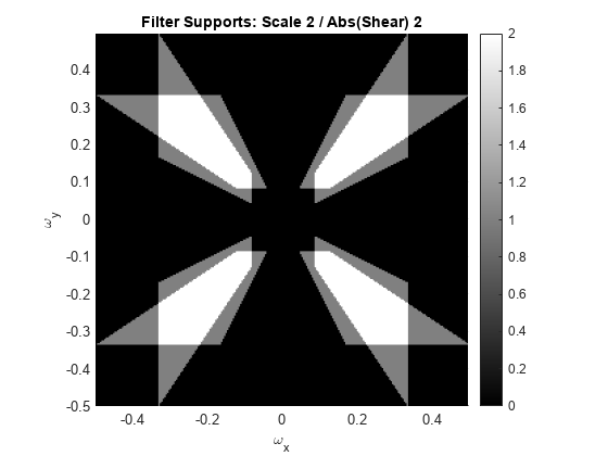
Plot the supports of all scale 2 shearlet filters with shear parameters equal to ±2. Areas where filter supports overlap have maximum brightness.

vScale = 2;
vShear = 2;
ind = find((scale==vScale).*(abs(shear)==vShear));
tmp = zeros(size(psi,1),size(psi,2));
for k=1:length(ind)
    tmp = tmp+(psi(:,:,ind(k))~=0);
end
surf(omegax,flip(omegay),double(tmp),'EdgeColor','none')
view(0,90)
xlabel('\omega_x')
ylabel('\omega_y')
str = sprintf('Filter Supports: Scale %d / Abs(Shear) %d',...
    vScale,vShear);
title(str)
axis equal
axis tight
colormap gray
colorbar

Figure contains an axes object. The axes object with title Filter Supports: Scale 2 / Abs(Shear) 2, xlabel omega indexOf x baseline, ylabel omega indexOf y baseline contains an object of type surface.

Input Arguments

collapse all

Shearlet system, specified as a shearletSystem object.

Output Arguments

collapse all

Fourier transforms of the shearlet filters defined by the shearlet system, returned as a 3-D real-valued array. The array size is M-by-N-by-K, where M and N are the first and second elements, respectively, of the ImageSize value of sls. K is the number of shearlets including the lowpass filter, K = numshears(sls) + 1. The first element in the third dimension of psi corresponds to the lowpass filter. The subsequent elements correspond to the shearlets.

The data type of psi matches the Precision value of the shearlet system.

Data Types: single | double

Scale parameters of the shearlet filters defined by the shearlet system, returned as a K-by-1 integer vector. K is the number of shearlets including the lowpass filter, K = numshears(sls) + 1. The first element of scale, −1, corresponds to the lowpass filter. The remaining elements of scale correspond to the shearlet filters.

The data type of scale matches the Precision value of the shearlet system.

Data Types: single | double

Shearing parameters of the shearlet filters defined by the shearlet system, returned as a K-by-1 integer vector. K is the number of shearlets including the lowpass filter, K = numshears(sls) + 1. The shear values at scale S range from −ceil(2^(S/2)) to ceil(2^(S/2)) inclusive. The first element of shear, 0, corresponds to the lowpass filter. The remaining elements of shear denote the shears for the corresponding shearlet filters.

The data type of shear matches the Precision value of the shearlet system.

Data Types: single | double

Frequency cones of the shearlet filters defined by the shearlet system, returned as a K-by-1 cell array of characters. K is the number of shearlets including the lowpass filter, K = numshears(sls) + 1. The first element of cone, 'X', corresponds to the lowpass filter. The remaining elements of cone are the frequency cones in which the corresponding shearlet filters have their frequency support.

For complex-valued shearlets, the frequency plane is divided into four cones: 'R' (right), 'T' (top), 'L' (left), and 'B' (bottom). For real-valued shearlets, the frequency cones are 'H' (horizontal) and 'V' (vertical).

Extended Capabilities

C/C++ Code Generation
Generate C and C++ code using MATLAB® Coder™.

Version History

Introduced in R2019b