Time-Delay Approximation in Continuous-Time Open-Loop Model

This example shows how to approximate delays in a continuous-time open-loop system using pade.

Padé approximation is helpful when using analysis or design tools that do not support time delays. Using too high an approximation order can result in numerical issues and possibly unstable poles. Therefore, avoid Padé approximations with order N>10.

Create sample open-loop system with an output delay.

s = tf('s');
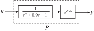
P = exp(-2.6*s)/(s^2+0.9*s+1);

P is a second-order transfer function (tf) object with a time delay.

Compute the first-order Padé approximation of P.

Pnd1 = pade(P,1)

Pnd1 =
 
             -s + 0.7692
  ----------------------------------
  s^3 + 1.669 s^2 + 1.692 s + 0.7692
 
Continuous-time transfer function.

This command replaces all time delays in P with a first-order approximation. Therefore, Pnd1 is a third-order transfer function with no delays.

Compare the frequency response of the original and approximate models using bodeplot.

bp = bodeplot(P,'-b',Pnd1,'-.r',{0.1,10});
bp.PhaseMatchingEnabled = 'on';
legend('Exact delay','First-Order Pade','Location','SouthWest');

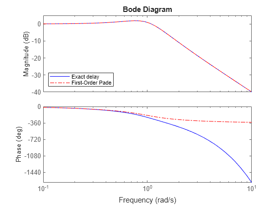
The magnitude of P and Pnd1 match exactly. However, the phase of Pnd1 deviates from the phase of P beyond approximately 1 rad/s.

Increase the Padé approximation order to extend the frequency band for which the phase approximation is good.

Pnd3 = pade(P,3);

Compare the frequency response of P, Pnd1, and Pnd3.

bp = bodeplot(P,'-b',Pnd3,'-.r',Pnd1,':k',{0.1 10})

bp = 
  BodePlot with properties:

                 Responses: [3x1 controllib.chart.response.BodeResponse]
           Characteristics: [1x1 controllib.chart.options.CharacteristicsManager]

             FrequencyUnit: "rad/s"
            FrequencyScale: "log"
             MagnitudeUnit: "dB"
            MagnitudeScale: "linear"
                 PhaseUnit: "deg"
          MagnitudeVisible: on
              PhaseVisible: on
      PhaseWrappingEnabled: off
       PhaseWrappingBranch: -180
      PhaseMatchingEnabled: off
    PhaseMatchingFrequency: 0
        PhaseMatchingValue: 0
        MinimumGainEnabled: off
          MinimumGainValue: 0

               GridVisible: off
                   Visible: on
                IOGrouping: "none"
              InputVisible: on
             OutputVisible: on

  Use GET to show all properties

bp.PhaseMatchingEnabled = 'on';
legend('Exact delay','Third-Order Pade','First-Order Pade',...
       'Location','SouthWest');

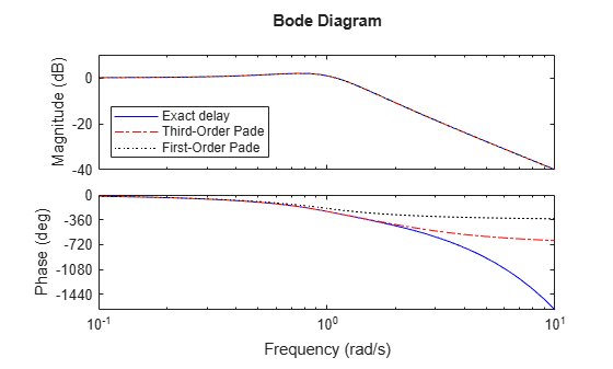
The phase approximation error is reduced by using a third-order Padé approximation.

Compare the time domain responses of the original and approximated systems using stepplot.

stepplot(P,'-b',Pnd3,'-.r',Pnd1,':k')
legend('Exact delay','Third-Order Pade','First-Order Pade',...
       'Location','Southeast');

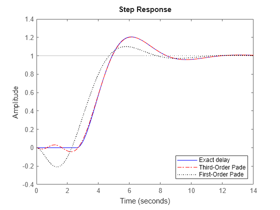
Using the Padé approximation introduces a nonminimum phase artifact ("wrong way" effect) in the initial transient response. The effect is quite pronounced in the first-order approximation, which dips significantly below zero before changing direction. The effect is reduced in the higher-order approximation, which more closely matches the exact system response.