Constructing and Working with ppform Splines

Constructing a ppform

A piecewise-polynomial is usually constructed by some command, through a process of interpolation or approximation, or conversion from some other form e.g., from the B-form, and is output as a variable. But it is also possible to make one up from scratch, using the statement

pp
= ppmak(breaks,coefs)

For example, if you enter pp=ppmak(-5:-1,-22:-11), or, more explicitly,

breaks = -5:-1;
coefs = -22:-11; pp = ppmak(breaks,coefs);

you specify the uniform break sequence -5:-1 and the coefficient sequence -22:-11. Because this break sequence has 5 entries, hence 4 break intervals, while the coefficient sequence has 12 entries, you have, in effect, specified a piecewise-polynomial of order 3 (= 12/4). The command

fnbrk(pp)

prints out all the constituent parts of this piecewise-polynomial, as follows:

breaks(1:l+1)
    -5 -4 -3 -2 -1  
coefficients(d*l,k)
     -22 -21 -20
     -19 -18 -17
     -16 -15 -14 
     -13 -12 -11
  pieces number l
    4 
order k 
  3 
dimension d of target
    1

Further, fnbrk can be used to supply each of these parts separately. But the point of Curve Fitting Toolbox™ spline functionality is that you usually need not concern yourself with these details. You simply use pp as an argument to commands that evaluate, differentiate, integrate, convert, or plot the piecewise-polynomial whose description is contained in pp.

Working With ppform Splines

Here are some functions for operations you can perform on a piecewise-polynomial.

`v = fnval(pp,x)`	Evaluates
`dpp = fnder(pp)`	Differentiates
`dirpp = fndir(pp,dir)`	Differentiates in the direction `dir`
`ipp = fnint(pp)`	Integrates
`fnmin(pp,[a,b])`	Finds the minimum value in given interval
`fnzeros(pp,[a,b])`	Finds the zeros in the given interval
`pj = fnbrk(pp,j)`	Pulls out the `j`th polynomial piece
`pc = fnbrk(pp,[a b])`	Restricts/extends to the interval [`a`..`b`]
`po = fnxtr(pp,order)`	Extends outside its basic interval by polynomial of specified order
`fnplt(pp,[a,b])`	Plots on given interval
`sp = fn2fm(pp,'B-')`	Converts to B-form
`pr = fnrfn(pp,morebreaks)`	Inserts additional breaks

Inserting additional breaks comes in handy when you want to add two piecewise-polynomials with different breaks, as is done in the command fncmb.

Example ppform

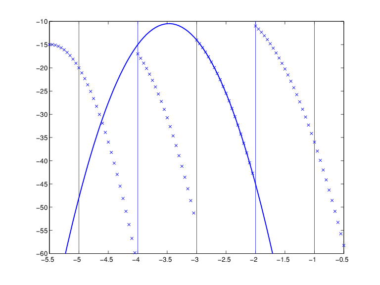
Execute the following commands to create and plot the particular piecewise-polynomial (ppform) described in the Constructing a ppform section.

Create the piecewise-polynomial with break sequence -5:-1 and coefficient sequence -22:-11:
```
pp=ppmak(-5:-1,-22:-11)
```

Create the basic plot:

x = linspace(-5.5,-.5,101);
plot(x, fnval(pp,x),'x')

Add the break lines to the plot:

breaks=fnbrk(pp,'b'); yy=axis; hold on
for j=1:fnbrk(pp,'l')+1
   plot(breaks([j j]),yy(3:4))
end

Superimpose the plot of the polynomial that supplies the third polynomial piece:
```
plot(x,fnval(fnbrk(pp,3),x),'linew',1.3)
set(gca,'ylim',[-60 -10]), hold off 
```

A Piecewise-Polynomial Function, Its Breaks, and the Polynomial Giving Its Third Piece

The plot shows a concave down parabola and five vertical lines. Between each pair of vertical lines, a different segment of the parabola is plotted with crosses.

The figure above is the final picture. It shows the piecewise-polynomial as a sequence of points and, solidly on top of it, the polynomial from which its third polynomial piece is taken. It is quite noticeable that the value of a piecewise-polynomial at a break is its limit from the right, and that the value of the piecewise-polynomial outside its basic interval is obtained by extending its leftmost, respectively its rightmost, polynomial piece.

While the ppform of a piecewise-polynomial is efficient for evaluation, the construction of a piecewise-polynomial from some data is usually more efficiently handled by determining first its B-form, i.e., its representation as a linear combination of B-splines.