Data Preparation for Neural Network Digital Predistortion Design

Since R2024a

This example shows how to prepare data for training a neural network digital predistortion (NN-DPD) system. The NN-DPD offsets the effects of nonlinearities in a power amplifier (PA). In this example, you:

1. Generate OFDM signals.

2. Send these OFDM signals through an real or simulated PA and measure the output.

3. Visualize the training data.

4. Preprocess the data for training an augmented real-valued time-delay neural network (ARVTDNN) [1].

Introduction

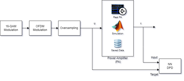
This diagram shows the setup for training an NN-DPD. Measure the input to the PA, $$u$$, and the output of the PA, $$x$$. To train the neural network as the inverse of the PA and use it as a DPD, use $$x$$ as the input signal and $$u$$ as the target signal. This architecture is also called indirect learning [2].

You can use three common data sources for training an NN-DPD, as shown in the Power Amplifier block:

• Real PA: For this source, you use a test and measurement device to collect PA measurements. For an example, see Power Amplifier Characterization (Communications Toolbox).

• Simulated PA: For this source, you use a simulated model of a neural network-based model, which was trained using captured data from a real PA, to simulate nonlinear effects of the PA. For an example, see Power Amplifier Modeling using Neural Networks (Communications Toolbox).

• Saved data: For this source, you use excitation and response data that you save directly from the PA.

Generate Oversampled OFDM Signals

Generate OFDM-based signals to excite the PA. This example uses a 5G-like OFDM waveform. Set the bandwidth of the signal to 100 MHz. Choosing a larger bandwidth signal causes the PA to introduce more nonlinear distortion and yields greater benefit from the addition of the DPD. Using the ofdmmod (Communications Toolbox) and qammod (Communications Toolbox) functions, generate six OFDM symbols, where each subcarrier carries a 16-QAM symbol. Save the 16-QAM symbols as a reference to calculate the EVM performance. To capture effects of higher order nonlinearities, the example oversamples the PA input by a factor of 5.

% Set random number generator seed for repeatable results. 
rng(123)

bw = 100e6;       % Hz
symPerFrame = 6;  % OFDM symbols per frame
M = 16;           % Each OFDM subcarrier contains a 16-QAM symbol
osf = 5;          % Oversampling factor for PA input

% OFDM parameters
ofdmParams = helperOFDMParameters(bw,osf);
numDataCarriers = (ofdmParams.fftLength - ofdmParams.NumGuardBandCarrier - 1);
nullIdx = [1:ofdmParams.NumGuardBandCarrier/2+1 ...
  ofdmParams.fftLength-ofdmParams.NumGuardBandCarrier/2+1:ofdmParams.fftLength]';

% Random data
x = randi([0 M-1],numDataCarriers,symPerFrame);

% OFDM with 16-QAM in data subcarriers
qamRefSym = single(qammod(x, M));
txWaveTrain = single(ofdmmod(qamRefSym/osf,ofdmParams.fftLength,ofdmParams.cpLength, ...
  nullIdx,OversamplingFactor=osf));
qamRefSymTrain = qamRefSym;

The helperNNDPDGenerateOFDM.m file encapsulates this process in a single function. Use the helperNNDPDGenerateOFDM function to generate validation and testing transmitter waveforms.

[txWaveVal,qamRefSymVal] = helperNNDPDGenerateOFDM(ofdmParams,symPerFrame,M);
[txWaveTest,qamRefSymTest] = helperNNDPDGenerateOFDM(ofdmParams,symPerFrame,M);

Send Signals Through Power Amplifier

Select the data source for the system. This example uses an NXP™ Airfast LDMOS Doherty PA, which connects to a local NI™ VST, as described in the Power Amplifier Characterization (Communications Toolbox) example. To obtain the real PA measurements, set the dataSource to NVIST. If you do not have access to a real PA, run the example with simulated PA data or data saved for specific inputs. If you set datasource to Simulated PA, the example uses a neural network PA model, which is trained as explained in the Power Amplifier Modeling using Neural Networks (Communications Toolbox) example. If you set dataSource to Saved data, the example downloads the files that contain data files collected from a PA using specific inputs.

dataSource = "Simulated PA";
if strcmp(dataSource,"Saved data")
  helperNNDPDDownloadData("dataprep")
end

Pass the signal through the PA and record the output signal. Lower target input power values can cause less distortion. Select a target input power level that is high enough to push the PA into its nonlinear region but lower than the maximum output of the power supply. The signals pass through a 30 dB attenuator before entering the measurement device. Also, the measurement device normalizes the measured signals to the same scale and synchronizes them.

if strcmp(dataSource,"NI VST")
  targetInputPower = 5; % dBm
  VST = helperVSTDriver('VST_01');
  VST.DUTExpectedGain     = 29;                % dB
  VST.ExternalAttenuation = 30;                % dB
  VST.DUTTargetInputPower = targetInputPower;  % dBm
  VST.CenterFrequency     = 3.7e9;             % Hz

  % Send the signals to the PA and collect the outputs
  Fs = ofdmParams.SampleRate;
  [paOutputTrain,measInfo] = helperNNDPDPAMeasure(txWaveTrain,Fs,VST);
  linearGainPA = measInfo.LinearGain;
  paOutputVal = helperNNDPDPAMeasure(txWaveVal,Fs,VST);
  paOutputTest = helperNNDPDPAMeasure(txWaveTest,Fs,VST);
elseif strcmp(dataSource,"Simulated PA")
  linearGainPA = 24.5;
  load paModelNN.mat netPA memDepthPA nonlinearDegreePA scalingFactorPA
  paPreprocessor = helperNNDPDInputPreprocessor(memDepthPA,nonlinearDegreePA);

  paInputFearures = paPreprocessor(txWaveTrain*scalingFactorPA);
  Y = predict(netPA,paInputFearures);
  paOutputTrain = complex(Y(:,1), Y(:,2)) / scalingFactorPA;

  
  paInputFearures = paPreprocessor(txWaveVal*scalingFactorPA);
  Y = predict(netPA,paInputFearures);
  paOutputVal = complex(Y(:,1), Y(:,2)) / scalingFactorPA;

  paInputFearures = paPreprocessor(txWaveTest*scalingFactorPA);
  Y = predict(netPA,paInputFearures);
  paOutputTest = complex(Y(:,1), Y(:,2)) / scalingFactorPA;
else
  load nndpdTrainingDataOct23 txWaveTrain qamRefSymTrain paOutputTrain ...
    txWaveVal qamRefSymVal paOutputVal txWaveTest qamRefSymTest paOutputTest ...
    linearGainPA
end

Visualize Training Data

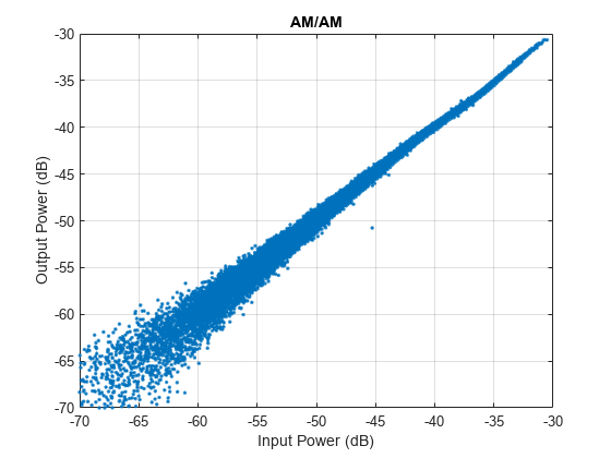
Plot AM/AM characteristics of the PA with the gain versus input power.

figure
plot(20*log10(abs(txWaveTrain)),20*log10(abs(paOutputTrain)),'.')
xlim([-70 -30])
ylim([-70 -30])
grid on
title("AM/AM")
xlabel("Input Power (dB)")
ylabel("Output Power (dB)")

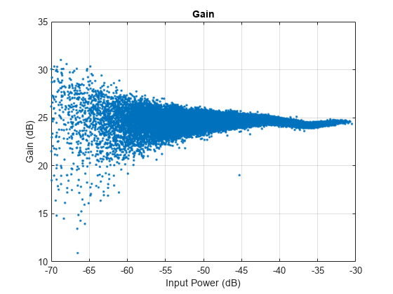
For a better view, focus on gain versus input power instead of output power versus input power and plot the data again.

paGain = 20*log10(abs(paOutputTrain))-20*log10(abs(txWaveTrain))+linearGainPA;
figure
plot(20*log10(abs(txWaveTrain)),paGain,'.')
xlim([-70 -30])
ylim([10 35])
grid on
title("Gain")
xlabel("Input Power (dB)")
ylabel("Gain (dB)")

The helperNNDPDPowerAmplifier System object™ combines all three PA data source implementations. Set DataSource property to NI VST for real PA measurements. Set DataSource property to Simulated PA to run the PA input signals through an NN-PA model. Set DataSource property to Saved data to use data collected from the PA using specific inputs. This setting works only with the specific input signals and is provided to demonstrate the results obtained using the specific real PA with the specific trained NN-DPD.

Preprocess Input Data

Preprocessing the training data involves scaling and feature extraction.

Scaling

Normalizing the input signal avoids the gradient explosion problem and ensures that the neural network converges to a better solution ([3], [4]). Normalization requires obtaining a unity standard deviation and zero mean. For this example, the communication signals already have zero mean, so normalize only the standard deviation. Later, denormalize the NN-DPD output values by using the same scaling factor.

scalingFactor = 1/std(txWaveTrain);

paInputTrainNorm = txWaveTrain*scalingFactor;
paOutputTrainNorm = paOutputTrain*scalingFactor;
paInputValNorm = txWaveVal*scalingFactor;
paOutputValNorm = paOutputVal*scalingFactor;
txWaveTestNorm = txWaveTest*scalingFactor;

Feature Extraction

This example prepares the augmented inputs used in the augmented real-valued time-delay neural network DPD structure (ARVTDNN) [1]. The ARVTDNN uses the structure of the memory polynomial model to generate features and use as inputs to the NN. The memory polynomial model is commonly used in the behavioral modeling and predistortion of PAs with memory effects. This equation:

$\mathit{x}\left(\mathit{n}\right)=\mathit{f}\left(\mathit{u}\left(\mathit{n}\right)\right)=\sum _{\mathit{m}=0}^{\mathit{M}-1}\sum _{\mathit{k}=0}^{\mathit{K}-1}{\mathit{c}}_{\mathit{m}}\mathit{u}\left(\mathit{n}-\mathit{m}\right){\left|\mathit{u}\left(\mathit{n}-\mathit{m}\right)\right|}^{\mathit{k}}$

where $$m$$ is the memory depth and $$k$$ is the nonlinearity order.

In this model, the output is a function of the delayed versions of the input signal, $$u(n)$$. It also powers of the amplitudes of $$u(n)$$ and its delayed versions. Use $$u(n-m)$$ and $$|u(n-m){|}^k$$ terms as inputs. To account for the memory in the PA model, the ${\mathit{I}}_{\mathrm{in}}$/${\mathit{Q}}_{\mathrm{in}}$ samples and $$m$$ delayed versions are part of the input the PA model. Also, to account for the nonlinearity of the PA, this model feeds the amplitudes of the ${\mathit{I}}_{\mathrm{in}}$/${\mathit{Q}}_{\mathrm{in}}$ samples up to the $$k^{th}$$ power as input.

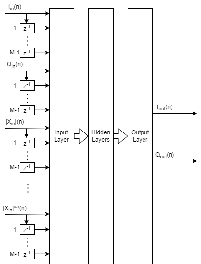
These processed time samples act as features for the neural network:

$$\begin{array}{l}[\mathrm{\Re }\left(\mathit{u}\left[\mathit{n}-\mathit{M}+1\right]\right)\mathrm{\Re }\left(\mathit{u}\left[\mathit{n}-\mathit{M}+2\right]\right)\cdots \mathrm{\Re }\left(\mathit{u}\left[\mathit{n}\right]\right)...\\ \mathrm{\Im }\left(\mathit{u}\left[\mathit{n}-\mathit{M}+1\right]\right)\mathrm{\Im }\left(\mathit{u}\left[\mathit{n}-\mathit{M}+2\right]\right)\cdots \mathrm{\Im }\left(\mathit{u}\left[\mathit{n}\right]\right)...\\ |\mathit{u}\left[\mathit{n}-\mathit{M}+1\right]{|\mathit{u}\left[\mathit{n}-\mathit{M}+1\right]|}^2\cdots {|\mathit{u}\left[\mathit{n}-\mathit{M}+1\right]|}^{\mathit{k}}...\\ |\mathit{u}\left[\mathit{n}-\mathit{M}+2\right]{|\mathit{u}\left[\mathit{n}-\mathit{M}+2\right]|}^2\cdots {|\mathit{u}\left[\mathit{n}-\mathit{M}+2\right]|}^{\mathit{k}}...\\ \cdots \\ |\mathit{u}\left[\mathit{n}\right]{|\mathit{u}\left[\mathit{n}\right]|}^2\cdots {|\mathit{u}\left[\mathit{n}\right]|}^{\mathit{k}}]\end{array}$$

where x is the input to the DPD, $$\mathrm{\Re }$$ is the real part and I, $$\mathrm{\Im }$$ is the imaginary part or Q. The total number of features per time sample is $$2m+(k-1)m$$. Assume $$m$$ and $$k$$ are 5.

The Neural Network for Digital Predistortion Design-Offline Training (Communications Toolbox) example uses indirect training, where DPD is trained as the inverse of the PA. So, use PA output as DPD training input and PA input as DPD training output.

memoryDepth = 5;
nonlinearDeg = 5;
numFeatures = 2*memoryDepth+(nonlinearDeg-1)*memoryDepth

numFeatures = 30

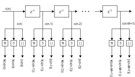
To generate features that depend on the previous samples, create a buffer in the form of a tapped delay line and initialize to all zeros. Process each tap of the delay line to obtain real and imaginary parts (I and Q), and the magnitude of the sample.

xBuffer = zeros(1,memoryDepth);

Take the $$1^{st}$$ through $$(k-1{)}^{th}$$ power of the magnitude of the current and delayed samples. Use a vector from $$1$$ to $$k-1$$. The following code demonstrates the implementation.

degrees = 1:nonlinearDeg-1;
disp(reshape(abs((1:memoryDepth).').^degrees,1,[]))

     1     2     3     4     5     1     4     9    16    25     1     8    27    64   125     1    16    81   256   625

The following code shows the full input processing loop. For each time step, update the buffer and then concatenate real, imaginary, and magnitude powers to form the features vector.

numSamples = size(txWaveTrain,1);
inputTrainFeatures = zeros(numSamples,numFeatures);
x = paOutputTrainNorm;
for p = 1:numSamples
  % Feed from the end of the buffer
  xBuffer = [xBuffer(1,2:end), x(p,1)];
  inputTrainFeatures(p,:) = [real(xBuffer), imag(xBuffer), reshape(abs(xBuffer.').^degrees,1,[])];
end

dpdTrainOutput = [real(paInputTrainNorm) imag(paInputTrainNorm)];

Generate Validation and Testing Data

Since the data preprocessor needs buffers to calculate the output, use a System object to implement the preprocessor. First define nontunable public properties to store the memory depth and nonlinearity order. Set initial values to 1. Define the output data type with a default value of single-precision. For more information see, Property Attributes.

properties (Nontunable)
  MemoryDepth = 1
  NonlinearityOrder = 1
  OutputDataType (1,1) string {mustBeMember(OutputDataType,["double","single"])} = "single"
end

Define private properties to the store number of features, nonlinearity degrees, and tapped delay line buffer.

properties (Access=private)
  Buffer
  NumFeatures
  NonlinearityPowers
end

Set up private properties in the setupImpl method.

function setupImpl(obj,~)
  obj.NonlinearityPowers = 1:obj.NonlinearityOrder-1;
  obj.NumFeatures = 2*obj.MemoryDepth ...
    +(obj.NonlinearityOrder-1)*obj.MemoryDepth;
end

Initialize the tapped delay line in the resetImpl method.

function resetImpl(obj)
  obj.Buffer = zeros(1,obj.MemoryDepth,obj.OutputDataType);
end

Process the input signal, $$x$$, in the stepImpl method.

function y = stepImpl(obj,x)
  numSamples = size(x,1);
  y = zeros(numSamples,obj.NumFeatures,obj.OutputDataType);
  for p = 1:numSamples
    obj.Buffer = [obj.Buffer(2:end), x(p,1)];
    y(p,:) = [real(obj.Buffer), imag(obj.Buffer), ...
      reshape(abs(obj.Buffer)'.^obj.NonlinearityPowers,1,[])];
  end
end

Full implementation of the preprocessor is in the helperNNDPDInputPreprocessor.m file.

Create two input preprocessors to generate validation and testing data.

prepVal = helperNNDPDInputPreprocessor(memoryDepth,nonlinearDeg);
prepTest = helperNNDPDInputPreprocessor(memoryDepth,nonlinearDeg);

inputFeaturesVal = prepVal(paOutputValNorm);
whos inputFeaturesVal

  Name                       Size               Bytes  Class     Attributes

  inputFeaturesVal      131520x30            15782400  single              

dpdOutputVal = [real(paInputValNorm) imag(paInputValNorm)];
whos dpdOutputVal

  Name                   Size              Bytes  Class     Attributes

  dpdOutputVal      131520x2             1052160  single              

inputFeaturesTest = prepTest(txWaveTestNorm);

Save Training Data

Save the measured PA input and output signals to use in the next example. Do not save the processed data to minimize storage usage. Instead, process the data during training and testing.

disp("Saving training data and information...")

Saving training data and information...

save savedData txWaveTrain qamRefSymTrain paOutputTrain ...
  txWaveVal qamRefSymVal paOutputVal txWaveTest qamRefSymTest paOutputTest ...
  linearGainPA ofdmParams osf M symPerFrame bw
disp(dir("savedData.mat"))

       name: 'savedData.mat'
     folder: '/tmp/Bdoc24a_2533273_1214866/tp9b4c38bd/deeplearning_shared-ex50726155'
       date: '16-Feb-2024 17:40:31'
      bytes: 5929540
      isdir: 0
    datenum: 7.3930e+05

Further Exploration

Proceed to the Neural Network for Digital Predistortion Design-Offline Training (Communications Toolbox) example.

Helper Functions

• helperNNDPDPAMeasure

• helperNNDPDInputPreprocessor

References

[1] Wang, Dongming, Mohsin Aziz, Mohamed Helaoui, and Fadhel M. Ghannouchi. “Augmented Real-Valued Time-Delay Neural Network for Compensation of Distortions and Impairments in Wireless Transmitters.” IEEE Transactions on Neural Networks and Learning Systems 30, no. 1 (January 2019): 242–54. https://doi.org/10.1109/TNNLS.2018.2838039.

[2] Paaso, Henna, and Aarne Mammela. “Comparison of Direct Learning and Indirect Learning Predistortion Architectures.” In 2008 IEEE International Symposium on Wireless Communication Systems, 309–13. Reykjavik: IEEE, 2008. https://doi.org/10.1109/ISWCS.2008.4726067.

[3] Morgan, Dennis R., Zhengxiang Ma, Jaehyeong Kim, Michael G. Zierdt, and John Pastalan. “A Generalized Memory Polynomial Model for Digital Predistortion of RF Power Amplifiers.” IEEE Transactions on Signal Processing 54, no. 10 (October 2006): 3852–60. https://doi.org/10.1109/TSP.2006.879264.

[4] Wu, Yibo, Ulf Gustavsson, Alexandre Graell i Amat, and Henk Wymeersch. “Residual Neural Networks for Digital Predistortion.” In GLOBECOM 2020 - 2020 IEEE Global Communications Conference, 01–06. Taipei, Taiwan: IEEE, 2020. https://doi.org/10.1109/GLOBECOM42002.2020.9322327.