Train Smaller Neural Network Using Knowledge Distillation
This example shows how to reduce the memory footprint of a deep learning network by using knowledge distillation.
Many real world applications of deep learning networks have memory constraints. For example, a large neural network might not fit in the memory of a small mobile device. Therefore, it is often important to be able to reduce the size of a network while retaining a high level of accuracy. Knowledge distillation is one approach to achieve this. This technique, proposed by Hinton et al [1], consists in using a large and accurate teacher network to teach a smaller student network to make accurate predictions. For more details see the section Knowledge Distillation Loss Function.
In this example you:
Load a data set of digit images for training, validation and testing.
Define and train a large convolutional teacher network.
Define and train a small convolutional student network using the standard cross-entropy loss.
Train a copy of the same convolutional student network using the knowledge distillation loss.
Compare the classification accuracy and size of the three networks.
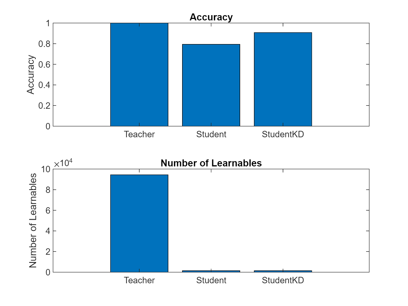
The chart below compares the accuracy of the three networks trained in this example and shows the large reduction in learnable parameters of the student architecture. You can see how the student network that was trained using knowledge distillation achieves significantly higher accuracy than the student network trained using the standard cross-entropy loss.
Load Training Data
Load the digits data as an image datastore using the imageDatastore function and specify the folder containing the image data.
unzip("DigitsData.zip")

imds = imageDatastore("DigitsData", ...
    IncludeSubfolders=true, ...
    LabelSource="foldernames");
Partition the data into training, testing, and validation sets. Allocate 60% of the data for training, 20% for testing, and 20% for validation using the splitEachLabel function.
[imdsTrain,imdsTest,imdsValidation] = splitEachLabel(imds,0.6,0.2,"randomize");The network used in this example requires input images of size 28-by-28-by-1. To automatically resize the training images, use an augmented image datastore. Specify additional augmentation operations to perform on the training images: randomly translate the images up to 5 pixels in the horizontal and vertical axes. Data augmentation helps prevent the network from overfitting and memorizing the exact details of the training images.
inputSize = [28 28 1];
pixelRange = [-5 5];

imageAugmenter = imageDataAugmenter( ...
    RandXTranslation=pixelRange, ...
    RandYTranslation=pixelRange);

augimdsTrain = augmentedImageDatastore(inputSize(1:2),imdsTrain,DataAugmentation=imageAugmenter);
To automatically resize the testing and validation images without performing further data augmentation, use augmented image datastores without specifying any additional preprocessing operations.
augimdsTest = augmentedImageDatastore(inputSize(1:2),imdsTest);
augimdsValidation = augmentedImageDatastore(inputSize(1:2),imdsValidation);
Determine the number of classes in the training data.
classes = categories(imdsTrain.Labels);
numClasses = numel(classes);
Define Teacher Network
Define the teacher network.
For image input, specify an image input layer with input size matching the training data.
Specify three convolution-batchnorm-ReLU blocks.
Pad the input to the convolution layers such that the output has the same size by setting the
Paddingoption to"same".The first convolution layer has 32 filters, the second one 64 and the last one 128.
Include max pooling layers to downsample the spatial dimension and improve shift invariance.
Include a global average pooling layer before the last fully connected layer to downsample the spatial dimension to one.
For classification, specify a fully connected layer with size matching the number of classes.
To convert the output to a probability distribution, use a softmax layer.
layersTeacher = [
    imageInputLayer(inputSize)

    convolution2dLayer(3,32,Padding="same")
    batchNormalizationLayer
    reluLayer

    maxPooling2dLayer(2, Stride=2)

    convolution2dLayer(3,64,Padding="same")
    batchNormalizationLayer
    reluLayer

    maxPooling2dLayer(2, Stride=2)

    convolution2dLayer(3,128,Padding="same")
    batchNormalizationLayer
    reluLayer

    globalAveragePooling2dLayer

    fullyConnectedLayer(numClasses)
    softmaxLayer];
Create a dlnetwork object from the layer array.
netTeacher = dlnetwork(layersTeacher)
netTeacher =
  dlnetwork with properties:

         Layers: [15×1 nnet.cnn.layer.Layer]
    Connections: [14×2 table]
     Learnables: [14×3 table]
          State: [6×3 table]
     InputNames: {'imageinput'}
    OutputNames: {'softmax'}
    Initialized: 1

  View summary with summary.
Define Student Network
Define the student network as a smaller similar version of the teacher model.
To do this, reduce the number of convolution-batchnorm-ReLU blocks as well as the number of filters in convolutional layers.
For image input, specify an image input layer with input size matching the training data.
Specify two convolution-batchnorm-ReLU blocks.
Pad the input to the convolution layers such that the output has the same size by setting the
Paddingoption to"same".The first convolution layer has 8 filters and the second one 16.
Include max pooling layers to downsample the spatial dimension and improve shift invariance.
Include a global average pooling layer before the last fully connected layer to downsample the spatial dimension to one.
For classification, specify a fully connected layer with size matching the number of classes.
To convert the output to a probability distribution, use a softmax layer.
layersStudent = [
    imageInputLayer(inputSize)

    convolution2dLayer(3,8,Padding="same")
    batchNormalizationLayer
    reluLayer

    maxPooling2dLayer(2, Stride=2)

    convolution2dLayer(3,16,Padding="same")
    batchNormalizationLayer
    reluLayer

    globalAveragePooling2dLayer

    fullyConnectedLayer(numClasses)
    softmaxLayer];
Create a dlnetwork object from the layer array to train the student network using a standard loss function.
netStudent = dlnetwork(layersStudent);
Create a copy of the dlnetwork object to train the student network using a knowledge distillation loss function.
netStudentKD = netStudent;
Compare Teacher and Student Architectures
Compare the number of learnable parameters of the teacher and student networks. To calculate the number of learnables of each network, use the numLearnables function, listed in the Number of Learnables Function section of the example.
numLearnables(netTeacher)
ans =
94410
numLearnables(netStudent)
ans =
1466
The number of learnable parameters of the student network is 1466. This is two order of magnitude smaller compared to the teacher network, which has 94,410 learnables.
The 98.4% reduction in learnable parameters of the student network compared to the teacher network results in a significantly smaller memory footprint and faster inference speed.
Specify Training Options
After defining the network architectures, specify the same training options for the teacher and student training loops for a fair comparison in accuracy.
Train the networks for 30 epochs, using stochastic gradient descent with momentum (SGDM) with an initial learning rate of 0.1 and piecewise drop factor of 0.1 every 10 epochs. Set the momentum parameter to 0.9. Set the mini-batch size to 128. Shuffle the data every epoch. Monitor the validation loss during training by specifying validation data and validation frequency. The validation data is not used to update the network weights. Turn on the training progress plot, and turn off the command window output. Compute and plot the accuracy metric at every iteration.
numEpochs = 30;
miniBatchSize = 128;
initialLearnRate = 0.1;
learnRateDropPeriod = 10;
learnRateDropFactor = 0.1;
momentum = 0.9;
validationFrequency = 100;

options = trainingOptions("sgdm", ...
    LearnRateSchedule="piecewise", ...
    InitialLearnRate=initialLearnRate, ...
    LearnRateDropPeriod=learnRateDropPeriod, ...
    LearnRateDropFactor=learnRateDropFactor, ...
    Momentum=momentum, ...
    MaxEpochs=numEpochs, ...
    Shuffle="every-epoch", ...
    MiniBatchSize=miniBatchSize, ...
    ValidationData=augimdsValidation, ...
    ValidationFrequency=validationFrequency, ...
    Verbose=false, ...
    Plots="training-progress", ...
    Metrics="accuracy");
Train Teacher Model
Train the teacher model netTeacher using the training data, the specified training options and a cross-entropy loss. By default, trainnet uses a GPU if one is available, otherwise, it uses a CPU. Using a GPU requires a Parallel Computing Toolbox™ license and a supported GPU device. For information about supported devices, see GPU Computing Requirements (Parallel Computing Toolbox). You can also specify the execution environment by using the ExecutionEnvironment name-value argument of trainingOptions.
The training progress plot shows the mini-batch loss and the validation loss and accuracy. For more information on the training progress plot, see Monitor Deep Learning Training Progress.
netTeacher = trainnet(augimdsTrain,netTeacher,"crossentropy",options);
Train Student Model
Train the student model netStudent using the training data, the specified training options and a cross-entropy loss. The training progress plot shows the mini-batch loss and the validation loss and accuracy.
netStudent = trainnet(augimdsTrain,netStudent,"crossentropy",options);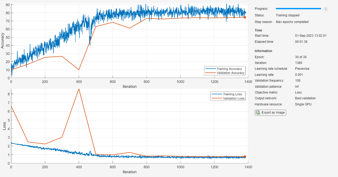
Train Student Model Using Knowledge Distillation
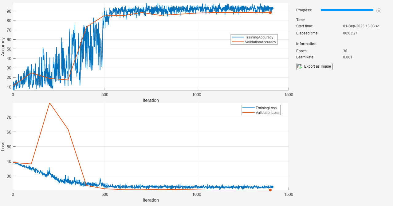
Train a separate copy of the student network, stored in the netStudentKD object, using the knowledge distillation loss.
To train using the knowledge distillation, use a custom training loop and define the custom loss function knowledgeDistLoss. This function is listed in the Knowledge Distillation Loss Function section at the end of the example. It takes as input the student network, the teacher network, a mini-batch of input data X with corresponding targets T, the temperature hyperparameter, and returns the knowledge distillation loss, the gradients of the loss with respect to the learnable parameters of the student network, and the student network state using knowledge distillation.
Create a minibatchqueue object that processes and manages mini-batches of images during training. For each mini-batch:
Use the custom mini-batch preprocessing function
preprocessMiniBatch(defined at the end of this example) to convert the labels to one-hot encoded variables.Format the image data with the dimension labels
"SSCB"(spatial, spatial, channel, batch). By default, theminibatchqueueobject converts the data todlarrayobjects with underlying typesingle. Do not format the class labels.Train on a GPU if one is available. By default, the
minibatchqueueobject converts each output to agpuArrayif a GPU is available.
Prepare the training and validation data.
mbq = minibatchqueue(augimdsTrain,...
    MiniBatchSize=miniBatchSize,...
    MiniBatchFcn=@preprocessMiniBatch,...
    MiniBatchFormat=["SSCB" ""]);

mbqVal = minibatchqueue(augimdsValidation, ...
    MiniBatchSize=miniBatchSize, ...
    MiniBatchFcn=@preprocessMiniBatch, ...
    MiniBatchFormat=["SSCB" ""]);
Initialize the velocity and learn rate parameters for the SGDM solver.
velocity = [];
learnRate = initialLearnRate;
Set the temperature hyperparameter of the knowledge distillation loss to four.
temperature = 4;
Calculate the total number of iterations for the training progress monitor.
numObservationsTrain = numel(imdsTrain.Files);
numIterationsPerEpoch = ceil(numObservationsTrain / miniBatchSize);
numIterations = numEpochs * numIterationsPerEpoch;
Initialize the TrainingProgressMonitor object. Because the timer starts when you create the monitor object, make sure that you create the object close to the training loop.
monitor = trainingProgressMonitor( ...
    Metrics=["TrainingLoss" "ValidationLoss" "TrainingAccuracy" "ValidationAccuracy"], ...
    Info=["Epoch", "LearnRate"], ...
    XLabel="Iteration");
Group the training and validation accuracy and loss plots.
groupSubPlot(monitor, "Accuracy", ["TrainingAccuracy" "ValidationAccuracy"]);
groupSubPlot(monitor, "Loss", ["TrainingLoss" "ValidationLoss"]);
Train the network using a custom training loop. Decrease the learn rate by 0.1 every 10 epochs. For each epoch, shuffle the data and loop over mini-batches of data. For each mini-batch:
Evaluate the model loss, gradients, and state using the
dlfevalandknowledgeDistLossfunctions and update the network state.Update the network parameters using the
sgdmupdatefunction.Update the loss, learn rate, and epoch values in the training progress monitor.
Update the validation loss plot every
validationFrequencyiterations.Stop if the Stop property is true. The Stop property value of the
TrainingProgressMonitorobject changes to true when you click the Stop button.
epoch = 0;
iteration = 0;

% Loop over epochs.
while epoch < numEpochs && ~monitor.Stop

    epoch = epoch + 1;

    % Shuffle data.
    shuffle(mbq);

    % Loop over mini-batches.
    while hasdata(mbq) && ~monitor.Stop

        iteration = iteration + 1;

        % Read mini-batch of data.
        [X,T] = next(mbq);

        % Evaluate the model gradients, state, and loss using dlfeval and the
        % knowledgeDistLoss function and update the network state.
        [loss,gradients,state] = dlfeval(@knowledgeDistLoss,netStudentKD,netTeacher,X,T,temperature);
        netStudentKD.State = state;

        % Update the network parameters using the SGDM optimizer.
        [netStudentKD,velocity] = sgdmupdate(netStudentKD,gradients,velocity,learnRate,momentum);

        % Record training loss and accuracy.
        Tdecode = onehotdecode(T,classes,1);
        scoresVal = predict(netStudentKD,X);

        Y = onehotdecode(scoresVal,classes,1);
        accuracyTrain = mean(Tdecode == Y);

        recordMetrics(monitor,iteration, ...
            TrainingLoss=loss, ...
            TrainingAccuracy=100*accuracyTrain);
        updateInfo(monitor,Epoch=epoch, LearnRate = learnRate);
        monitor.Progress = 100 * iteration/numIterations;

        % Perform validation step.
        if mod(iteration, validationFrequency) == 0 || iteration == 1

            % Compute the validation loss and accuracy.
            [lossVal, accuracyVal] = validationMetrics(netStudentKD, ...
                netTeacher,mbqVal,classes, ...
                augimdsValidation.NumObservations,temperature);

            % Update the validation loss and accuracy plots.
            recordMetrics(monitor,iteration, ...
                ValidationLoss=lossVal, ...
                ValidationAccuracy=100*accuracyVal);
        end
    end

    % Decrease the learning rate.
    if mod(epoch, learnRateDropPeriod) == 0
        learnRate = learnRate * learnRateDropFactor;
    end
end
Compare Model Accuracy
Test the classification accuracy of the three trained networks: the teacher network, the student network trained using cross-entropy loss and the student network trained using knowledge distillation. Calculate the accuracy of the networks using the testnet function.
accuracyTeacher = testnet(netTeacher,augimdsTest,"accuracy")accuracyTeacher = 99.9000
accuracyStudent = testnet(netStudent,augimdsTest,"accuracy")accuracyStudent = 77.7500
accuracyStudentKD = testnet(netStudentKD,augimdsTest,"accuracy")accuracyStudentKD = 90.4000
Compare the accuracy and the number of learnables of each network in a bar chart. To calculate the number of learnables of each network, use the numLearnables function, listed in the Number of Learnables Function section of the example.
figure
tiledlayout("flow")

nexttile
bar([accuracyTeacher accuracyStudent accuracyStudentKD])
xticklabels(["Teacher" "Student" "StudentKD"])
title("Accuracy")
ylabel("Accuracy")

nexttile
bar([numLearnables(netTeacher) numLearnables(netStudent) numLearnables(netStudentKD)])
xticklabels(["Teacher" "Student" "StudentKD"])
ylabel("Number of Learnables")
title("Number of Learnables")
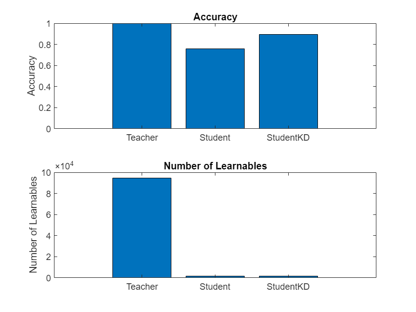
Notice how the student network trained using knowledge distillation benefits from the memory footprint reduction of the smaller student architecture while achieving a significantly higher accuracy than the student network trained using the standard cross-entropy loss.
Supporting Functions
Knowledge Distillation Loss Function
The knowledge distillation loss knowledgeDistLoss consists of a weighted average of the hard loss and the soft loss:
where:
lossHard is the cross-entropy loss between the student network outputs, YStudent, and the true labels Targets:
lossSoft: the cross-entropy loss between the student network logits logitsStudent and the teacher network logits logitsTeacher both transformed using the same softmax with temperature operation:
t is the temperature hyperparameter of the softmax with temperature operation.
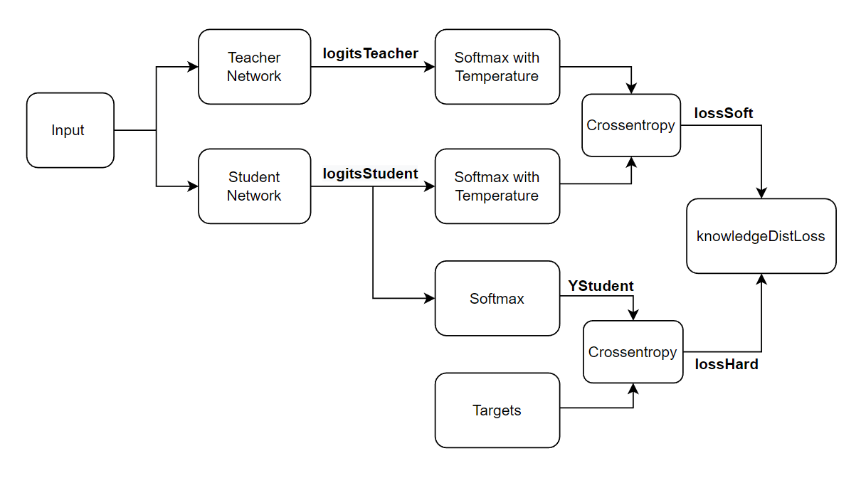
The knowledgeDistLoss function takes the student network, the teacher network, a mini-batch of input data X with corresponding targets T, and the temperature hyperparameter and returns the knowledge distillation loss, the gradients of the loss with respect to the learnable parameters of the student network, and the student network state. To compute the gradients automatically, use the dlgradient function.
function [lossKD,gradients,stateStudent] = knowledgeDistLoss(netStudent,netTeacher,X,T,temperature)

% Compute the logits and outputs of the student network.
[logitsStudent, YStudent, stateStudent] = forward(netStudent,X,Outputs=["fc" "softmax"]);

% Compute the logits of the teacher network.
logitsTeacher = predict(netTeacher,X,Outputs="fc");

% Compute the soft labels of both networks.
softLabelsStudent = softmaxWithTemperature(logitsStudent,temperature);
softLabelsTeacher = softmaxWithTemperature(logitsTeacher,temperature);

% Calculate the cross-entropy loss between soft labels.
lossSoft = crossentropy(softLabelsStudent,softLabelsTeacher);

% Calculate the cross-entropy loss between the student hard labels and the
% targets.
lossHard = crossentropy(YStudent,T);

% Combine the two losses into the knowledge distillation loss.
lossKD = lossSoft*temperature^2 + lossHard;

% Calculate gradients of loss with respect to the student network learnables.
gradients = dlgradient(lossKD,netStudent.Learnables);

end
Softmax with Temperature Function
The softmaxWithTemperature function takes a mini-batch of activations X and the temperature hyperparameter and converts the activations into a probability distribution computed using the softmax with temperature operation.
function softLabels = softmaxWithTemperature(X,temperature)

% Identify the channel dimension.
channelDim = finddim(X,"C");

% Apply softmax with temperature operation.
X = exp(X./temperature);
softLabels = X./sum(X,channelDim);

end
Validation Metrics Function
The validationMetrics function takes the student network, the teacher network, a minibatchqueue of input data mbqVal, the network classes, the total number of observations in the input data, and the temperature hyperparameter and returns the accuracy and knowledge distillation loss of the input validation dataset.
function [loss,accuracy] = validationMetrics(netStudent,netTeacher,mbqVal,classes,numObservations,temperature)

% Initialize total loss and accuracy
loss = 0;
accuracy = 0;

% Reset mini-batch queue.
reset(mbqVal);

% Loop over mini-batches.
while hasdata(mbqVal)
    [XVal, TVal] = next(mbqVal);

    % Compute the logits and hard labels of the student network.
    [logitsStudent, hardLabelsStudent] = predict(netStudent,XVal,Outputs=["fc", "softmax"]);

    % Compute the logits of the teacher network.
    logitsTeacher = predict(netTeacher,XVal,Outputs="fc");

    % Compute the soft labels of both networks.
    softLabelsStudent = softmaxWithTemperature(logitsStudent,temperature);
    softLabelsTeacher = softmaxWithTemperature(logitsTeacher,temperature);

    % Calculate the cross-entropy loss between soft labels.
    lossSoft = crossentropy(softLabelsStudent,softLabelsTeacher);

    % Calculate the cross-entropy loss between the student hard labels and the
    % targets.
    lossHard = crossentropy(hardLabelsStudent,TVal);

    % Combine the two losses into the knowledge distillation loss of a
    % single mini-batch.
    lossMb = lossSoft*temperature^2 + lossHard;

    % Decode probabilities into categorical arrays.
    predictions = onehotdecode(hardLabelsStudent,classes,1);
    targets = onehotdecode(TVal,classes,1);

    % Compute the accuracy of the mini-batch
    accuracyMb = mean(predictions == targets);

    % Calculate proportion of mini-batch elements to total number of
    % observations.
    weightMb = size(XVal, 4)/numObservations;

    % Update the validation dataset total loss and accuracy.
    loss = loss + weightMb * lossMb;
    accuracy = accuracy + weightMb * accuracyMb;
end

end
Mini-Batch Preprocessing Function
The preprocessMiniBatch function preprocesses a mini-batch of predictors and labels using the following steps:
Preprocess the images using the
preprocessMiniBatchPredictorsfunction.Extract the label data from the incoming cell array and concatenate into a categorical array along the second dimension.
One-hot encode the categorical labels into numeric arrays. Encoding into the first dimension produces an encoded array that matches the shape of the network output.
function [X,T] = preprocessMiniBatch(dataX,dataT)

% Preprocess predictors.
X = preprocessMiniBatchPredictors(dataX);

% Extract label data from cell and concatenate.
T = cat(2,dataT{1:end});

% One-hot encode labels.
T = onehotencode(T,1);

end
Mini-Batch Predictors Preprocessing Function
The preprocessMiniBatchPredictors function preprocesses a mini-batch of predictors by extracting the image data from the input cell array and concatenate into a numeric array. For grayscale input, concatenating over the fourth dimension adds a third dimension to each image, to use as a singleton channel dimension.
function X = preprocessMiniBatchPredictors(dataX)

% Concatenate.
X = cat(4,dataX{:});

end
Number of Learnables Function
The numLearnables function returns the total number of learnables in a network.
function N = numLearnables(net)

N = 0;
for i = 1:size(net.Learnables,1)
    N = N + numel(net.Learnables.Value{i});
end

end
References
[1] Hinton G, Vinyals O, Dean J. Distilling the knowledge in a neural network. arXiv preprint arXiv:1503.02531. 2015 Mar 9;2(7).
See Also
trainnet | compressNetworkUsingProjection | dlnetwork | minibatchqueue | dlarray | neuronPCA | ProjectedLayer