Verify Global Stability of ACAS Xu Neural Network Using Adaptive Mesh

Since R2026a

This example uses:

This example shows how to formally verify the global stability of ACAS Xu neural networks using an adaptive mesh algorithm. This example is step 4 in a series of examples that take you through formally verifying a set of neural networks that output steering advisories to aircraft to prevent them from colliding with other aircraft.

To run this example, open Verify and Deploy Airborne Collision Avoidance System (ACAS) Xu Neural Networks and navigate to Step4VerifyGlobalStabilityOfACASXuNeuralNetworkUsingAdaptiveMeshExample.m. This project contains all of the steps for this workflow. You can run the scripts in order or run each one independently.

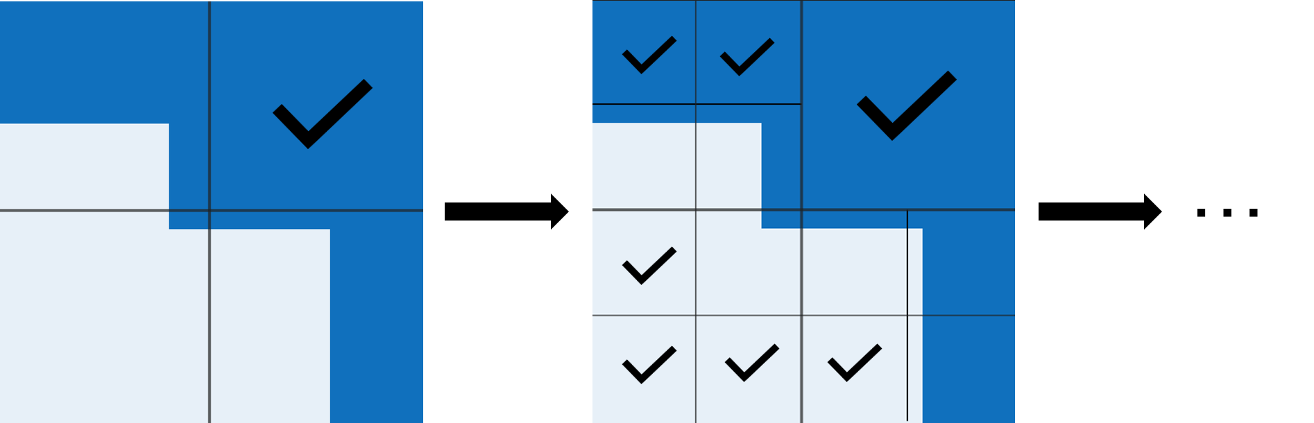
In this example, to verify the stability of the network, subdivide the operational design domain into smaller areas and check whether the network is stable in those areas. If the network is not stable in an area, further subdivide that area into even smaller areas. Continue to subdivide the ODD until either a specified minimum proportion of the ODD is determined stable, or you reach a specified minimum area size.

This figure illustrates the adaptive mesh process in a simplified 2-D ODD.

By default, the example uses a GPU if one is available. Using a GPU requires a Parallel Computing Toolbox™ license and a supported GPU device. For information on supported devices, see GPU Computing Requirements (Parallel Computing Toolbox). Otherwise, the example uses the CPU.

Adaptive Mesh Algorithm

In Verify Global Stability of ACAS Xu Neural Networks, when you split the ODD into eight equal hypercuboids per dimension, the verifyNetworkRobustness function returns unverified on 82% of the hypercuboids. You can increase the number of hypercuboids per dimension, but doing so can be computationally wasteful on the 18% of hypercuboids that already return verified at lower resolution.

In this example, incrementally increase the number of hypercuboids only in regions that were previously classified as unproven:

Verify the network stability of one of more hypercuboids.
If the verifyNetworkRobustness function returns unproven, split the hypercuboid into several smaller hypercuboids.
Repeat steps 1-2 until either:
1. A minimum proportion of the ODD is verified as stable.
2. The smallest hypercuboid size is smaller than a specified minimum hypercuboid size.

Whether this adaptive mesh approach is more efficient than the regular tiling approach described in Verify Global Stability of ACAS Xu Neural Networks depends on the available computational resources.

The regular tiling approach can be parallelized. Use this approach when you have access to a large number of workers.
The adaptive mesh approach reaches a given ODD resolution using a smaller total number of computations. However, the algorithm is iterative and cannot be completely parallelized.

Load ACAS Xu Neural Networks

Load and save the networks. The example prepares the networks as shown in Explore ACAS Xu Neural Networks.

acasXuNetworkFolder = fullfile(matlab.project.rootProject().RootFolder,".");
zipFile = matlab.internal.examples.downloadSupportFile("nnet","data/acas-xu-neural-network-dataset.zip");
filepath = fileparts(zipFile);
unzip(zipFile,acasXuNetworkFolder);
matFolder = fullfile(matlab.project.rootProject().RootFolder,"acas-xu-neural-network-dataset","networks-mat");
helpers.convertACASXuFromONNXAndSave(matFolder);

Verify Local Stability of Subset of ODD using Adaptive Mesh

Choose an ACAS Xu network by choosing the time until loss of vertical separation and the previous advisory. Load the network using the loadACASNetwork function, which is attached to this example as a supporting file. For more information on the different ACAS Xu neural networks, see Explore ACAS Xu Neural Networks.

timeUntilLossOfVerticalSeparation = 1;
previousAdvisory = 1;
net = helpers.loadACASNetwork(previousAdvisory,timeUntilLossOfVerticalSeparation);

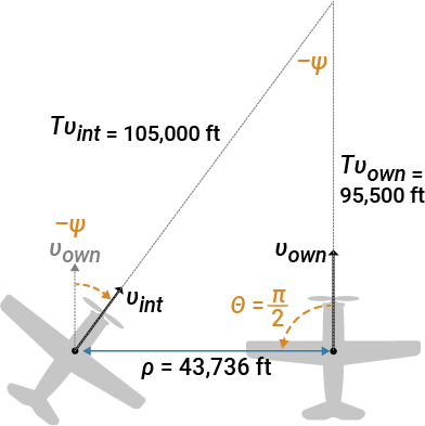
To illustrate the adaptive mesh algorithm, verify the stability of the network starting from the Left Abeam scenario and changing only the angles $θ$ and $ψ$ of the two aircraft. For more information on the different aircraft configurations, see Explore ACAS Xu Neural Networks.

To ensure that the adaptive mesh algorithm terminates, specify a minimum angle resolution minAngle. Do not split hypercuboids that are narrower than the minimum angle. If you increase minAngle, then a larger percentage of the ODD remains unproven. If you decrease minAngle, then the calculation takes longer to run.

minAngle = 0.01;

Specify the number of hypercuboids to analyze simultaneously. If you have a GPU and a Parallel Computing Toolbox license, then the example runs on the GPU and you can increase the mini-batch size.

miniBatchSize = 8192;

Define the input range. Set the initial distance, ownship velocity, and intruder velocity to the values corresponding to the Left Abeam scenario.

rho = 15000;     
vOwn = 954.6; 
vInt = 1050;

Allow the directions of the ownship and intruder to span all possible values.

thetaLower = -pi;
thetaUpper = pi; 
psiLower = -pi;
psiUpper = pi;

oddLower = [rho thetaLower psiLower vOwn vInt];
oddUpper = [rho thetaUpper psiUpper vOwn vInt];

Convert the ranges into dlarray objects.

oddLower = dlarray(oddLower,"BC");
oddUpper = dlarray(oddUpper,"BC");

To keep track of and manipulate the changing set of hypercuboids, this example uses two custom classes, CubeBatch and CubeBatchQueue, which are attached to this example as supporting files. For details on the class implementations, view the class implementation files.

>> edit helpers.CubeBatch
>> edit helpers.CubeBatchQueue

Create a CubeBatch object that contains a single hypercuboid spanning the input range.

cubes = helpers.CubeBatch(oddLower,oddUpper);

Create an empty CubeBatch object to keep track of the verified hypercuboids.

verifiedCubes = helpers.CubeBatch;

Create a CubeBatchQueue object and add the hypercuboid to the queue by using the enqueue function.

cubeQueue = helpers.CubeBatchQueue;
enqueue(cubeQueue,cubes);

Initialize the total number of hypercuboids, the labels of the verified hypercuboids, and the centers of the hypercuboids.

numHypercuboids = 0;
verifiedLabelBatch = [];
hypercuboidCenters = [];

Initialize adaptive mesh progress monitor by using the adaptiveMeshProgressMonitor function, which is defined at the bottom of this example.

adaptiveMeshProgressMonitor;

Run the adaptive mesh algorithm.

While the queue is not empty, verify the stability of all hypercuboids in the queue.

If the verification result for a hypercuboid is unproven, partition the hypercuboid into smaller hypercuboids and add them to the queue by using the cubeRefineAndUpdateQueue function, which is attached to this example as a supporting file. Remove any hypercuboid narrower than minAngle from the queue.

while ~isempty(cubeQueue)
    cubes = getCubes(cubeQueue,miniBatchSize);

    % Evaluate the network issued advisory at the hypercuboid centers
    centers = getCenters(cubes);
    hypercuboidCenters = [hypercuboidCenters extractdata(centers)]; %#ok<AGROW>

    advisory = predict(net,centers);
    [~,idxLabel] = max(extractdata(advisory));

    % Verify stability by using network predicted labels as the ground truth
    results = verifyNetworkRobustness(net,cubes.xLower,cubes.xUpper,idxLabel,MiniBatchSize=miniBatchSize);
    idxVerified = (results == "verified");
    idxUnproven = (results == "unproven");
    
    % Extract the verified hypercuboids
    verifiedMiniBatch  = getSubset(cubes,idxVerified);
    verifiedLabel     = idxLabel(idxVerified);
    verifiedLabelBatch = [verifiedLabelBatch verifiedLabel]; %#ok<AGROW>    
    verifiedCubes  = addSubset(verifiedCubes,verifiedMiniBatch);

    % Update the figure with the verified hypercuboids
    xlVerified = extractdata(verifiedMiniBatch.xLower);
    xuVerified = extractdata(verifiedMiniBatch.xUpper);
    sideLengths = xuVerified - xlVerified;
    for kk = 1:getNumCubes(verifiedMiniBatch)
        hold on
        rectangle(...
            Position=[xlVerified(2,kk) xlVerified(3,kk) sideLengths(2,kk) sideLengths(3,kk)], ...
            FaceColor=[getClassColors(verifiedLabel(kk)) 0.05], ... 
            EdgeColor="none");
    end
    hold off
    drawnow

    % Further divide hypercuboids that return unproven results
    unprovenCubes = getSubset(cubes,idxUnproven);
    helpers.bisectAndUpdateQueue(cubeQueue,unprovenCubes,minAngle);

    % Count the number of processed hypercuboids
    numHypercuboids = numHypercuboids + getNumCubes(cubes);
end

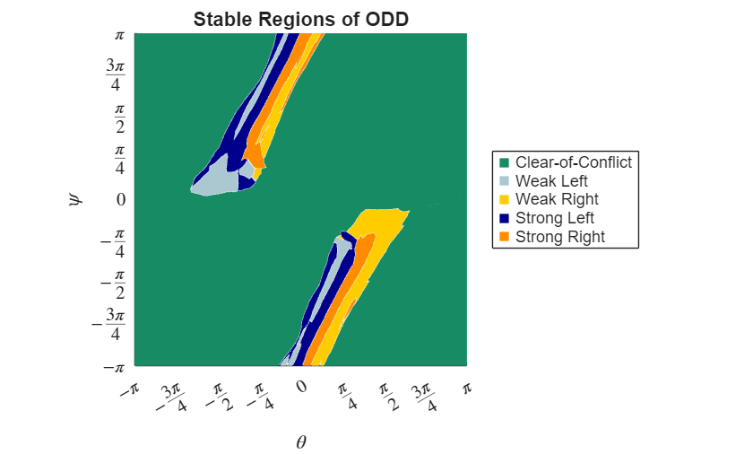
The adaptive mesh progress plot shows the results of the adaptive mesh algorithm.

As expected, the network output is antisymmetric. When you reflect both aircraft from right to left, $θ \to - θ$ and $ψ \to - ψ$ , the advisories change from Weak Right to Weak Left, Strong Right to Strong Left, and so on.
Large regions of the ODD are connected within the same class. This means that the network generalizes well in these regions.
There is a small, enclosed region in which the network advises Strong Right, bounded by Weak Right and Clear-of-Conflict regions. The network may not be trustworthy in this region, necessitating further analysis or retraining.
There are several decision boundaries in this subset of the ODD. The network behavior near these decision boundaries is highly nonlinear, which makes it difficult to understand the network stability and generalization without this global analysis.

Compare Network Prediction to Stability Analysis

Calculate the network output at random points inside the different regions of the ODD to confirm the stability analysis agrees with the true class at those points.

Investigate the regions that separated by the emergence of class boundaries by picking an arbitrary point in each region.

samplePoints = [
    [rho -3.00  3.00 vOwn vInt];  % Clear-of-Conflict
    [rho -1.50  1.00 vOwn vInt];  % Strong Left
    [rho -0.78  2.10 vOwn vInt];  % Weak Left
    [rho -0.78  1.57 vOwn vInt];  % Strong Right
    [rho -0.39  1.97 vOwn vInt];  % Weak Right
    [rho  0.70 -1.57 vOwn vInt];  % Strong Left
    [rho  0.78 -0.78 vOwn vInt];  % Weak Left
    [rho  0.90 -1.57 vOwn vInt];  % Strong Right
    [rho  1.57 -0.78 vOwn vInt];  % Weak Right
    [rho  0.95 -1.97 vOwn vInt];  % Strong Right
    ];
sampleAdvisory = predict(net,samplePoints);
sampleAdvisory = scores2label(sampleAdvisory,helpers.classNames)

sampleAdvisory = 10×1 categorical array
    "Clear-of-Conflict"
    "Strong Left"
    "Weak Left"
    "Strong Right"
    "Weak Right"
    "Strong Left"
    "Weak Left"
    "Strong Right"
    "Weak Right"
    "Strong Right"

The class labels in each region match those from the global stability analysis.

Compute Proportion of ODD by Class

Calculate the proportion of the ODD that has been proven stable as well as the total number of hypercuboids.

totalVolume = prod(oddUpper(2:3) - oddLower(2:3));
verifiedCubeVolume = sum(prod(verifiedCubes.xUpper(2:3,:) - verifiedCubes.xLower(2:3,:)));
disp("Stable proportion of ODD: " + extractdata(verifiedCubeVolume / totalVolume));

Stable proportion of ODD: 0.99007

disp("Number of hypercuboids: " + numHypercuboids);

Number of hypercuboids: 45565

Plot the proportion of the analyzed subset of the ODD by class by using the plotClassProportion function, which is defined at the bottom of this example.

plotClassProportion(verifiedLabelBatch,verifiedCubes,totalVolume);

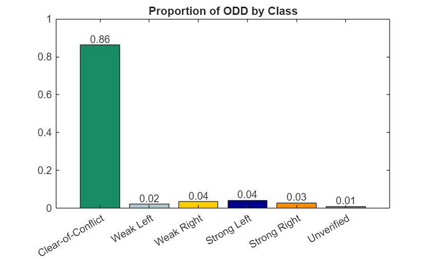
The unverified results, which represent a small proportion of the ODD, contain the decision boundaries.

Plot Hypercuboid Density

To visualize how much the network output changes in different regions of the ODD, plot the density of hypercuboids resulting from the adaptive mesh algorithm by using the plotHypercuboidDensity function, which is defined at the bottom of this example.

plotHypercuboidDensity(hypercuboidCenters)

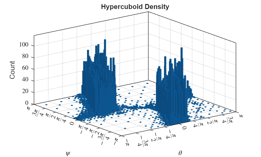
High bars indicate a large number of hypercuboids, which indicates the presence of decision boundaries.

Supporting Functions

`adaptiveMeshProgressMonitor`

The adaptiveMeshProgressMonitor function initializes the adaptive mesh progress plot.

function adaptiveMeshProgressMonitor
figure
axis equal
xlim([-pi pi])
ylim([-pi pi])
xticks(-pi:pi/4:pi)
yticks(-pi:pi/4:pi)
tickLabels = {'$-\pi$','$-\frac{3\pi}{4}$','$-\frac{\pi}{2}$','$-\frac{\pi}{4}$', ...
    '$0$','$\frac{\pi}{4}$','$\frac{\pi}{2}$','$\frac{3\pi}{4}$','$\pi$'};

xticklabels(tickLabels)
yticklabels(tickLabels)
set(gca,TickLabelInterpreter="latex");

xlabel("$\theta$",Interpreter="latex")
ylabel("$\psi$",Interpreter="latex")
title("Stable Regions of ODD")
grid on

for ii = 1:5
    hold on
    plot(-100,-100,"square", ...
        Color=getClassColors(ii), ...
        MarkerFaceColor=getClassColors(ii), ...
        MarkerEdgeColor=getClassColors(ii));
end
hold off
legend(helpers.classNames,Location="eastoutside");
end

`plotClassProportion`

The plotClassProportion function plots the percentage of the analyzed subset of the ODD that corresponds to each advisory class.

function plotClassProportion(labelVerified,verifiedCubes,totalVolume)
propVerifiedVolumePerClass = zeros(1,5);
for idxLabel = 1:5
    predictClassIdx = (labelVerified == idxLabel);
    verifiedCubeVolumePerClass = sum(prod(verifiedCubes.xUpper(2:3,predictClassIdx) - verifiedCubes.xLower(2:3,predictClassIdx)));    
    propVerifiedVolumePerClass(idxLabel) = verifiedCubeVolumePerClass / totalVolume;
end
propVerifiedVolumePerClass(end+1) = 1 - sum(propVerifiedVolumePerClass);

figure
b = bar([helpers.classNames; "Unverified"],...
    propVerifiedVolumePerClass);
b.FaceColor = "flat";
for idx = 1:5
    b.CData(idx,:) = getClassColors(idx);
end
b.CData(6,:) = [0.5, 0.5, 0.5];
ylim([0 1])
text(1:length(propVerifiedVolumePerClass),propVerifiedVolumePerClass,num2str(propVerifiedVolumePerClass',"%.2f"),"vert","bottom","horiz","center");
title("Proportion of ODD by Class")
end

`plotHypercuboidDensity`

The plotHypercuboidDensity function plots the number of hypercuboids in each area of the analyzed subsection of the ODD.

function plotHypercuboidDensity(hypercuboidCenters)
figure
nbins = 100;
histogram2(hypercuboidCenters(2,:),hypercuboidCenters(3,:),nbins)
xlim([-pi pi])
ylim([-pi pi])
xticks(-pi:pi/4:pi)
yticks(-pi:pi/4:pi)
tickLabels = ["$-\pi$","$-\frac{3\pi}{4}$","$-\frac{\pi}{2}$","$-\frac{\pi}{4}$", ...
    "$0$","$\frac{\pi}{4}$","$\frac{\pi}{2}$","$\frac{3\pi}{4}$","$\pi$"];
xticklabels(tickLabels)
yticklabels(tickLabels)
set(gca,TickLabelInterpreter="latex");
xlabel("$\theta$",Interpreter="latex")
ylabel("$\psi$",Interpreter="latex")
zlabel("Count")
title("Hypercuboid Density")
end

`getClassColors`

The getClassColors function defines plotting colors for each advisory class.

function classColours = getClassColors(idx)
classColours = [
    [ 0.0902    0.5490    0.3922];... % Clear-of-Conflict (green)
    [ 0.6706    0.7843    0.8196];... % Weak Left (light-blue)
    [ 1.0000    0.8000         0];... % Weak Right (light-orange)
    [      0         0    0.5451];... % Strong Left (dark-blue)
    [ 1.0000    0.5490         0];... % Strong Right (dark-orange)
    ];
classColours = classColours(idx,:);
end