FFT
Compute fast Fourier transform (FFT)
Libraries:
DSP HDL Toolbox /
Transforms
Description
The FFT block provides two architectures that implement the algorithm for FPGA and ASIC applications. You can select an architecture that optimizes for either throughput or area.
Streaming Radix 2^2— Use this architecture for high-throughput applications. This architecture supports scalar or vector input data. You can achieve gigasamples-per-second (GSPS) throughput, also called super sample rates, using vector input. Since 2025a, this architecture also supports specifying the FFT size by using an input port, when you use scalar input data.Burst Radix 2— Use this architecture for a minimum resource implementation, especially with large fast-Fourier-transform (FFT) sizes. Your system must be able to tolerate bursty data and higher latency. This architecture supports only scalar input data.
The block accepts real or complex data, provides hardware-friendly control signals, and optional output frame control signals.
Note
You can also generate HDL code for this hardware-optimized algorithm, without creating a Simulink® model, by using the DSP HDL IP Designer app. The app provides the same interface and configuration options as the Simulink block.
Examples
Implement an inverse fast Fourier transform (IFFT) by using a forward FFT block.
Instead of deploying a dedicated IFFT block, this design reuses an FFT block to calculate the inverse FFT by swapping the real and imaginary parts of the data both before and after the FFT operation. With this implementation, you can reuse a single FFT block to perform both FFT and IFFT computations in hardware, as long as you do not require both operations at the same time. This approach is well suited for FPGA or ASIC designs that have limited hardware resources.
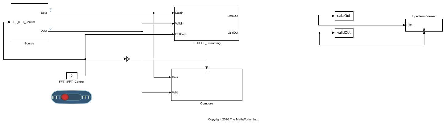
Model Overview
The top-level model includes these features:
Input Signal Generation
IFFT Implementation Using FFT with Real/Imaginary Swapping
Result Visualization
The model operates on complex data and uses a streaming interface with control signals to indicate when the data is valid. The system processes 8 samples per cycle and implements a 512-point FFT/IFFT.
The FFTIFFT_Streaming subsystem contains the FFT block from the DSP HDL Toolbox™ library and swapping logic.
Use the toggle switch to select between FFT and IFFT modes. Set FFT_IFFT_Control signal to 0 for IFFT mode or to 1 for FFT mode. The switch enables or disables the swapping logic inside the FFTIFFT_Streaming subsystem and modifies the source output.
The Spectrum Viewer subsystem reorders the output samples to account for the bit-reversed order from the FFT block, and plots the output. The model also exports output data to the workspace.
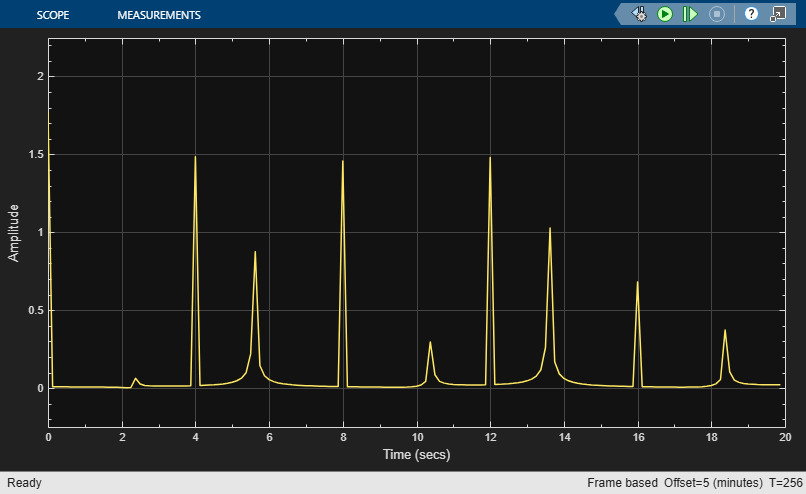
modelname = 'FFTIFFTHDL_Streaming';
open_system(modelname);
% Set scope time interval.
scopePath = [modelname '/Spectrum Viewer/Time Scope'];
set_param(scopePath, 'TimeSpan', num2str(20));
Generate Input Signal
The source subsystem generates frames of 512 complex input samples in the time-domain. In IFFT mode, the source returns the FFT of the time-domain signal. The MATLAB® code generates the signal, casts it to a fixed-point type, and generates a corresponding valid signal. The valid signal indicates when each input sample is available for processing, ensuring synchronization with the FFT block.
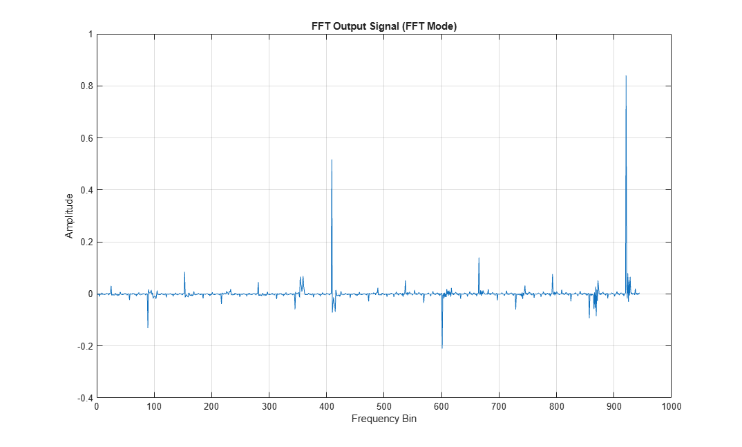
FFT Operation
When you set the FFT_IFFT_Control signal to 1 (FFT mode), the model computes the 512-point FFT of the input frame and outputs the frequency-domain representation of the signal.
Set FFT_IFFT_Control to FFT mode and run the model to capture the FFT output. The plot shows the real part of the FFT output for the current frame. You can use this output to analyze the frequency content of the input signal.
set_param([modelname '/FFT_IFFT_Control'], 'Value', '1');
sim(modelname);
Visualize the FFT output.
FFTOutput = squeeze(dataOut(:,:,validOut));
figure;
plot(real(FFTOutput(:)));
xlabel('Frequency Bin');
ylabel('Amplitude');
title('FFT Output Signal (FFT Mode)');
grid on;
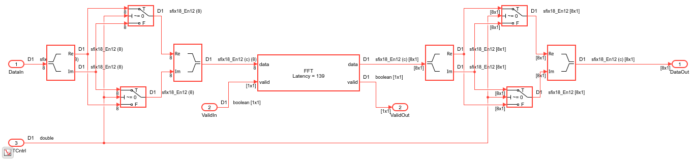
Inverse FFT Algorithm
The FFTIFFT_Streaming subsystem computes the IFFT by using a forward FFT block and swapping the real and imaginary parts.
Input Swapping: The model separates the complex input signal into real and imaginary components, then swaps and recombines the components to create a new complex data signal. The valid signal remains aligned with the swapped data.
FFT Processing: The model passes the swapped complex signal to a forward FFT block configured for a length of 512 samples. The FFT block produces output in bit-reversed order.
Output Swapping: The model splits the FFT output into real and imaginary parts, then swaps and recombines the components a second time.
Mathematically, this process is:
![$$x'[n] = \mathrm{Im}(x[n]) + j\,\mathrm{Re}(x[n])$$](../../examples/dsphdl/win64/CalculateInverseFFTUsingAForwardFFTBlockHDLExample_eq05484494437333196802.png)
![$$X'[k] = \mathrm{FFT}(x'[n])$$](../../examples/dsphdl/win64/CalculateInverseFFTUsingAForwardFFTBlockHDLExample_eq10114284411887094959.png)
![$$y[k] = \mathrm{Im}(X'[k]) + j\,\mathrm{Re}(X'[k])$$](../../examples/dsphdl/win64/CalculateInverseFFTUsingAForwardFFTBlockHDLExample_eq07043485408952949663.png)
Now, set FFT_IFFT_Control to IFFT mode and run the model.
open_system([modelname '/FFTIFFT_Streaming']);
set_param([modelname '/FFT_IFFT_Control'],'Value','0');
sim(modelname);
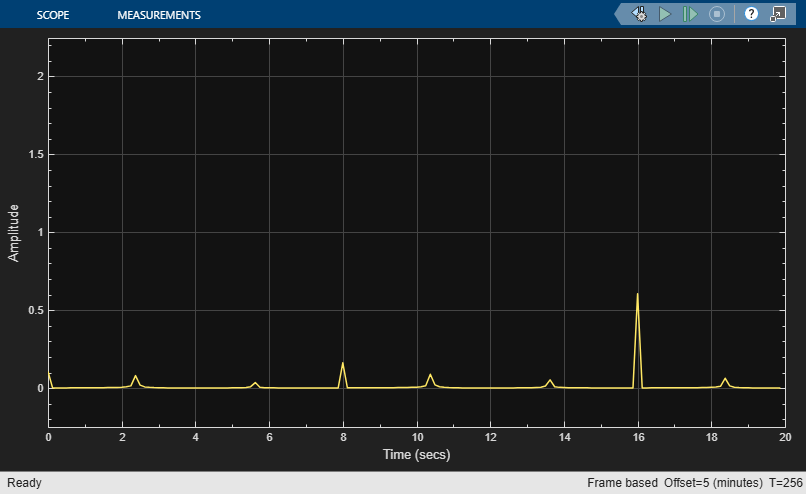
Visualize IFFT Result
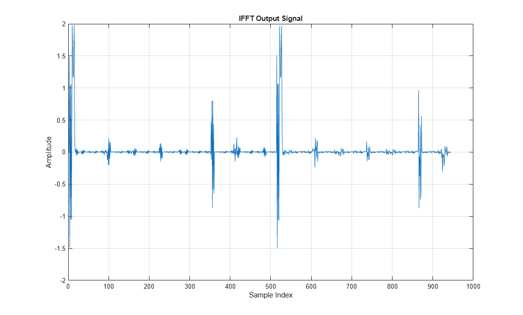
The figure shows the time-domain signal reconstructed by the IFFT operation. The x-axis shows the sample index, and the y-axis shows the amplitude of each sample. Each stem corresponds to a time-domain sample obtained after calculating the IFFT of the frequency-domain signal with swapped real and imaginary parts.
IFFTOutput = squeeze(dataOut(:,:,validOut));
figure;
plot(real(IFFTOutput(:)));
xlabel('Sample Index');
ylabel('Amplitude');
title('IFFT Output Signal');
grid on;
Compare with Reference IFFT
To verify the implementation, compare the output of the FFT-based IFFT method with a standard IFFT block from DSP HDL Toolbox™. The plots show both outputs for comparison.
validDataRef = squeeze(refOut(:,:,refValidOut));
figure;
plot(real(IFFTOutput(:)),'b'); % Blue line for IFFTOutput
hold on;
stem(real(validDataRef(:)),'r','filled','Marker','o');
xlabel('Sample Index');
ylabel('Amplitude');
title('Comparison: FFT-based IFFT vs. Reference IFFT');
legend('FFT-based IFFT','Reference IFFT');
grid on;
hold off;
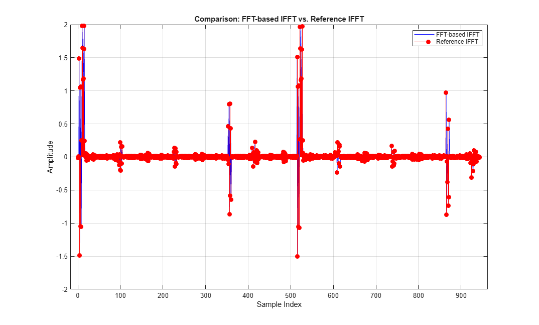
The output matches the result of a dedicated IFFT implementation. This technique enables efficient resource sharing and suits FPGA and ASIC designs where minimizing logic usage is important.
More Design Options
An alternative way to implement the IFFT using an FFT block is the conjugate method. You can perform the IFFT by finding the complex conjugate of the input signal, then running it through the FFT block, finding the complex conjugate of the FFT output, and finally dividing the result by the FFT length (N). The method shown in this example is a slightly simpler algorithm with less logic.
Extended Examples

Implement FFT Algorithm for FPGA
Implement two hardware-optimized FFT architectures in Simulink.

Frequency-Domain Filtering in HDL
Implement a filter in the frequency domain. The filter is built with the FFT and IFFT blocks from DSP HDL Toolbox™.

Automatic Delay Matching for the Latency of FFT Block
Programmatically obtain the latency of an FFT block in a model for use in delay matching.
Ports
Input
Output
Parameters
Algorithms
The streaming Radix 2^2 architecture implements a low-latency architecture. It saves resources compared to a streaming Radix 2 implementation by factoring and grouping the FFT equation. The architecture has log4(N) stages. Each stage contains two single-path delay feedback (SDF) butterflies with memory controllers. When you use vector input, each stage operates on fewer input samples, so some stages reduce to a simple butterfly, without SDF.

The first SDF stage is a regular butterfly. The second stage multiplies the outputs of the first stage by –j. To avoid a hardware multiplier, the block swaps the real and imaginary parts of the inputs, and again swaps the imaginary parts of the resulting outputs. Each stage rounds the result of the twiddle factor multiplication to the input word length. The twiddle factors have two integer bits, and the rest of the bits are used for fractional bits. The twiddle factors have the same bit width as the input data, WL. The twiddle factors have two integer bits, and WL-2 fractional bits.
If you enable scaling, the algorithm divides the result of each butterfly stage by 2. Scaling at each stage avoids overflow, keeps the word length the same as the input, and results in an overall scale factor of 1/N. If scaling is disabled, the algorithm avoids overflow by increasing the word length by 1 bit at each stage. The diagram shows the butterflies and internal word lengths of each stage, not including the memory.

The burst Radix 2 architecture implements the FFT by using a single complex butterfly multiplier. The algorithm cannot start until it has stored the entire input frame, and it cannot accept the next frame until computations are complete. The output ready port indicates when the algorithm is ready for new data. The diagram shows the burst architecture, with pipeline registers.

When you use this architecture, your input data must comply with the ready backpressure signal.
The algorithm processes input data only when the input valid port is 1. Output data is valid only when the output valid port is 1.
When the optional input reset port is 1, the algorithm stops the current calculation and clears all internal states. The algorithm begins new calculations when reset port is 0 and the input valid port starts a new frame.
This diagram shows the input and output valid input values for contiguous scalar input data, streaming Radix 2^2 architecture, an FFT length of 1024, and a vector size of 16.
The diagram also shows the optional start and end outputs that indicate frame boundaries. If you enable the start output, the start output pulses for one cycle with the first valid output of the frame. If you enable the end output, the end output pulses for one cycle with the last valid output of the frame.
If you apply continuous input frames, the output will also be continuous after the initial latency.

The valid input can be noncontiguous. The algorithm processes data accompanied by a validsignal as it arrives, and stores the resulting data until a frame is filled. Then the algorithm returns contiguous output samples in a frame of N (FFT length) cycles. This diagram shows noncontiguous input and contiguous output for an FFT length of 512 and a vector size of 16.

When you use the burst architecture, you cannot provide the next frame of input data until
memory space is available. The ready output indicates when the
algorithm can accept new input data. The algorithm sets the ready
output to 1 (true) when it can accept data, and to
0 (false) when it is processing and cannot accept
more data. If the upstream part of your design has continuous input data and synchronously
reacts to ready before halting input, then one extra cycle of input
data can arrive at the port. This data is the beginning of the next frame. To support
synchronous control logic, the block reserves room to store this extra data while processing
the current frame. For more detail about this extra data, see the annotated waveform in the
Latency
section.

Variable-size FFT designs must also respect the ready signal. When
you load a new FFT length, the algorithm sets ready to
0 (false) while it updates internal logic with the
new size. If the algorithm is processing a previous frame when you load a new FFT size, the
algorithm finishes the frame and then updates internal logic to use the new size.
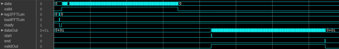
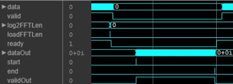
The first waveform shows loading the input size before any frame is processed. The
algorithm sets the ready signal to 0
(false) for 4 cycles while it updates internal logic with the new
size, and then sets ready to 1
(true) again. The waveform shows new input data and
valid set to 1 (true) once
the ready signal is 1 (true)
again.
The next waveform shows loading a new FFT size while a frame is processing. When you load
a new size, the algorithm sets the ready signal to 0
(false). You can continue to provide the rest of the current input
frame. The block sets ready to 1
(true) when it has completed the current frame and updated the
internal logic with the new size. You can apply the next frame, of the new size, once the
ready signal is 1 (true).
The latency varies with the FFT length and input vector size. After you update the model, the block icon displays the latency. The displayed latency is the number of cycles between the first valid input and the first valid output, assuming the input is contiguous. To obtain this latency programmatically, see Automatic Delay Matching for the Latency of FFT Block.
When using the burst
architecture, if the upstream part of your design has continuous input data and synchronously
reacts to ready before halting input, then one extra cycle of input data
can arrive at the port. This data is the beginning of the next frame. To support synchronous
control logic, the block reserves room to store this extra data while processing the current
frame. Due to this one cycle advance, the observed latency of the later frames (cycles from
first input valid to first output valid) is one cycle
shorter than the reported latency. The number of cycles between when ready
port is 0 (false) and the output
valid port is 1 (true) is always
latency – FFTLength.

References
[1] Algnabi, Y.S, F.A. Aldaamee, R. Teymourzadeh, M. Othman, and M.S. Islam. “Novel architecture of pipeline Radix 2^2 SDF FFT Based on digit-slicing technique.” 10th IEEE International Conference on Semiconductor Electronics (ICSE). 2012, pp. 470–474.