Determine Asymptotic Behavior of Markov Chain
This example shows how to compute the stationary distribution of a Markov chain, estimate its mixing time, and determine whether the chain is ergodic and reducible. The example also shows how to remove periodicity from a chain without compromising asymptotic behavior.
Consider this theoretical, right-stochastic transition matrix of a stochastic process.
Create the Markov chain that is characterized by the transition matrix P. Plot a digraph of the chain and indicate transition probabilities by using edge colors.
P = [ 0   0  1/2 1/4 1/4  0   0 ;
      0   0  1/3  0  2/3  0   0 ;
      0   0   0   0   0  1/3 2/3;
      0   0   0   0   0  1/2 1/2;
      0   0   0   0   0  3/4 1/4;
     1/2 1/2  0   0   0   0   0 ;
     1/4 3/4  0   0   0   0   0 ];
mc = dtmc(P);

figure;
graphplot(mc,'ColorEdges',true);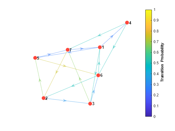
Because the transition matrix is right stochastic, the Markov chain has a stationary distribution such that .
Determine whether the Markov chain is irreducible.
tfRed = isreducible(mc)
tfRed = logical
   0
tfRed = 0 indicates that the chain is irreducible. This result implies that is unique.
Determine whether the Markov chain is ergodic.
tfErg = isergodic(mc)
tfErg = logical
   0
tfErg = 0 indicates that the chain is not ergodic. This result implies that is not a limiting distribution for an arbitrary initial distribution.
You can determine whether a Markov chain is periodic in two ways.
Chains that are irreducible and not ergodic are periodic. The results in the previous section imply that the Markov chain is periodic.
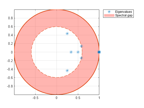
Inspect a plot of the eigenvalues on the complex plane. An eigenvalue plot indicates whether the Markov chain is periodic, and the plot reveals the period of the chain.
Plot the eigenvalues of the Markov chain on the complex plane.
figure;
eigplot(mc);

Notable features of the eigenvalue plot include:
The bold asterisk is the Perron-Frobenius eigenvalue. It has a magnitude of 1 and is guaranteed for nonnegative transition matrices.
All eigenvalues at roots of unity indicate the periodicity. Because three eigenvalues are on the unit circle, the chain has a period of 3.
The spectral gap is the area between the circumference of the unit circle and the circumference of the circle with a radius of the second largest eigenvalue magnitude (SLEM). The size of the spectral gap determines the mixing rate of the Markov chain.
In general, the spectrum determines structural properties of the chain.
Compute the stationary distribution of the Markov chain.
xFix = asymptotics(mc)
xFix = 1×7

    0.1300    0.2034    0.1328    0.0325    0.1681    0.1866    0.1468
xFix is the unique stationary distribution of the chain, but is not the limiting distribution for an arbitrary initial distribution.
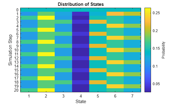
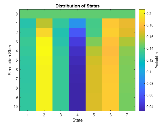
Visualize two evolutions of the state distribution of the Markov chain by using two 20-step redistributions. For the first redistribution, use the default uniform initial distribution. For the second redistribution, specify an initial distribution that puts all the weight on the first state.
X1 = redistribute(mc,20);
figure;
distplot(mc,X1);
X2 = redistribute(mc,20,'X0',[1 0 0 0 0 0 0]);
figure;
distplot(mc,X2);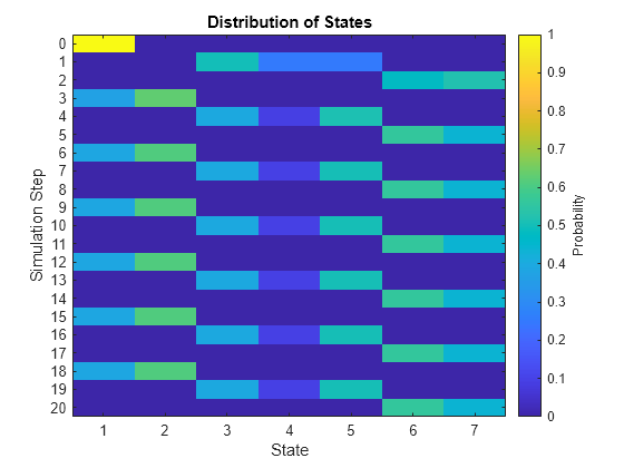
In the figures, periodicity is apparent and prevents the state distribution from settling. Also, different initial values yield different evolutions.
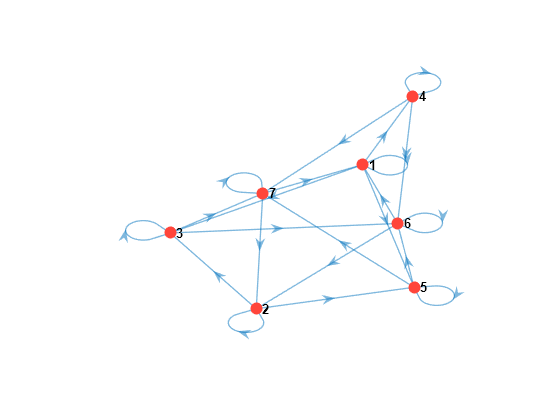
Remove periodicity from the Markov chain by transforming the chain to a "lazy" chain. Plot a digraph of the lazy chain. Determine whether the lazy chain is irreducible and ergodic.
lc = lazy(mc);

figure;
graphplot(lc);
tfRedLC = isreducible(lc)
tfRedLC = logical
   0
tfErgLC = isergodic(lc)
tfErgLC = logical
   1
Observe the self-loops in the digraph. To remove periodicity, the lazy chain enforces state persistence. The lazy chain is irreducible and ergodic.
Plot the eigenvalues of the lazy chain on the complex plane.
figure;
eigplot(lc);
The lazy chain does not have any eigenvalues at roots of unity, except for the Perron-Frobenius eigenvalue. Therefore, the lazy chain has a period of 1. Because the spectral gap of the lazy chain is thinner than the spectral gap of the untransformed chain, the lazy chain mixes more slowly than the untransformed chain.
Compute the stationary distribution of the lazy chain.
xFixLC = asymptotics(lc)
xFixLC = 1×7

    0.1300    0.2034    0.1328    0.0325    0.1681    0.1866    0.1468
xFixLC is the unique stationary distribution of the chain, and it is the limiting distribution given an arbitrary initial distribution. Also, xFixLC and xFix are identical.
Visualize the evolution of the state distribution of the lazy chain by using a 10-step redistribution.
XLC = redistribute(lc,10);

figure;
distplot(lc,XLC)
The state distribution evolves from a uniform distribution to the stationary distribution in fewer than 10 time steps. Observe that colors at the final step match the values in xFixLC.