asymptotics
Determine Markov chain asymptotics
Description
Examples
Consider this theoretical, right-stochastic transition matrix of a stochastic process.
Create the Markov chain that is characterized by the transition matrix P.
P = [ 0   0  1/2 1/4 1/4  0   0 ;
      0   0  1/3  0  2/3  0   0 ;
      0   0   0   0   0  1/3 2/3;
      0   0   0   0   0  1/2 1/2;
      0   0   0   0   0  3/4 1/4;
     1/2 1/2  0   0   0   0   0 ;
     1/4 3/4  0   0   0   0   0 ];
mc = dtmc(P);
Plot a directed graph of the Markov chain. Indicate the probability of transition by using edge colors.
figure;
graphplot(mc,'ColorEdges',true);
Determine the stationary distribution of the Markov chain.
xFix = asymptotics(mc)
xFix = 1×7

    0.1300    0.2034    0.1328    0.0325    0.1681    0.1866    0.1468
Because xFix is a row vector, it is the unique stationary distribution of mc.
Create a five-state transition matrix of empirical counts by generating a block diagonal matrix composed of discrete uniform draws.
m = 100; % Maximal count
rng(1); % For reproducibility
P = blkdiag(randi(100,2) + 1,randi(100,3) + 1)
P = 5×5

    43     2     0     0     0
    74    32     0     0     0
     0     0    16    36    43
     0     0    11    41    70
     0     0    20    55    22
Create and plot a digraph of the Markov chain that is characterized by the transition matrix P.
mc = dtmc(P);

figure;
graphplot(mc)

Determine the stationary distribution and mixing time of the Markov chain.
[xFix,tMix] = asymptotics(mc)
xFix = 2×5

    0.9401    0.0599         0         0         0
         0         0    0.1497    0.4378    0.4125
tMix =
0.8558
Rows of xFix correspond to the stationary distributions of the two independent recurrent classes of mc.
Create separate Markov chains representing the recurrent subchains of mc.
mc1 = subchain(mc,1);
mc2 = subchain(mc,3);
mc1 and mc2 are dtmc objects. mc1 is the recurrent class containing state 1, and mc2 is the recurrent class containing state 3.
Compare the mixing times of the subchains.
[x1,t1] = asymptotics(mc1)
x1 = 1×2

    0.9401    0.0599
t1 =
0.7369
[x2,t2] = asymptotics(mc2)
x2 = 1×3

    0.1497    0.4378    0.4125
t2 =
0.8558
mc1 approaches its stationary distribution more quickly than mc2.
Create a "dumbbell" Markov chain containing 10 states in each "weight" and three states in the "bar."
Specify random transition probabilities between states within each weight.
If the Markov chain reaches the state in a weight that is closest to the bar, then specify a high probability of transitioning to the bar.
Specify uniform transitions between states in the bar.
rng(1,"twister"); % For reproducibility
w = 10;                              % Dumbbell weights
DBar = [0 1 0; 1 0 1; 0 1 0];        % Dumbbell bar
DB = blkdiag(rand(w),DBar,rand(w));  % Transition matrix

% Connect dumbbell weights and bar
DB(w,w+1) = 1;
DB(w+1,w) = 1;
DB(w+3,w+4) = 1;
DB(w+4,w+3) = 1;

mc = dtmc(DB);
Visualize the transition matrix using a heatmap.
figure
imagesc(mc.P)
axis square
colorbar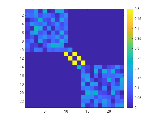
Plot a directed graph of the Markov chain. Suppress node labels.
figure
h = graphplot(mc);
h.NodeLabel = {};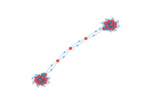
Plot the eigenvalues of the dumbbell chain.
figure
eigplot(mc)
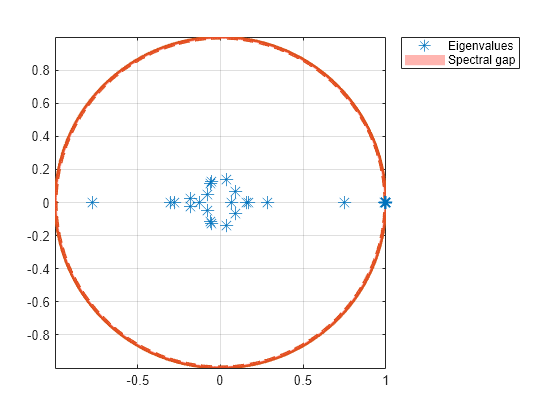
The thin, red disc in the plot shows the spectral gap (the difference between the two largest eigenvalue moduli). The spectral gap determines the mixing time of the Markov chain. Large gaps indicate faster mixing, whereas thin gaps indicate slower mixing. In this case, the spectral gap is thin, indicating a long mixing time.
Estimate the mixing time of the dumbbell chain and determine whether the chain is ergodic.
[~,tMix] = asymptotics(mc)
tMix =
85.3258
tf = isergodic(mc)
tf = logical
   1
On average, the time it takes for the total variation distance between any initial distribution and the stationary distribution to decay by a factor of is about 85 steps.
Input Arguments
Output Arguments
References
[1] Gallager, R.G. Stochastic Processes: Theory for Applications. Cambridge, UK: Cambridge University Press, 2013.
[2] Horn, R., and C. R. Johnson. Matrix Analysis. Cambridge, UK: Cambridge University Press, 1985.
[3] Seneta, E. Non-negative Matrices and Markov Chains. New York, NY: Springer-Verlag, 1981.
Version History
Introduced in R2017b