Markov Chain Modeling
Discrete-Time Markov Chain Object Framework Overview
The dtmc
object framework provides basic tools for modeling and analyzing discrete-time
Markov chains. The object supports chains with a finite number of states that evolve
in discrete time with a time-homogeneous transition structure.
dtmc identifies each Markov chain with a
NumStates-by-NumStates transition matrix
P, independent of initial state
x0 or initial distribution of states
π0. You can specify
P as either a right-stochastic matrix or a matrix of
empirical counts.
As a right-stochastic matrix:
Pij is the nonnegative probability of a transition from state i to state j.
Each row of P sums to 1.
describes the evolution of the state distribution from time t to time t + 1.
The state distribution at time t, πt is a row vector of length
NumStates.As a matrix of empirical counts, Pij is the observed number of times state i transitions to state j. The
dtmcobject normalizes the rows of P so that it is a right-stochastic matrix.
The mcmix
function is an alternate Markov chain object creator; it generates a chain with a
specified zero pattern and random transition probabilities. mcmix is
well suited for creating chains with different mixing times for testing
purposes.
To visualize the directed graph, or digraph, associated with a chain, use the
graphplot object function. graphplot is similar to the plot object function of a
MATLAB®
digraph object, but it includes
additional functionality for analyzing Markov chain structure. Parameter settings
highlight communicating classes (that is, strongly connected
components of the digraph) and specific characteristics affecting convergence, such
as recurrence, transience, and periodicity. You can highlight transition
probabilities in P by coloring the graph edges using heatmap intensities.

To visualize large-scale structure in the chain, graphplot
can condense communicating classes to representative nodes. This option is based on
the condensation object function of a
digraph object.
The classify
object function is a numerical analog of class highlighting in the graph. classify
returns characteristics of the communicating classes that determine limiting
behavior. State classification combines graph-theoretic algorithms, such as the
bfsearch (breadth-first search)
object function of a MATLAB
graph object, but with more direct
matrix computations specific to Markov chain theory. The subchain
method allows you to extract specific communicating classes from the chain for
further analysis.
The isreducible and isergodic object functions give concise summaries of chain
structure. Together, they provide necessary and sufficient conditions for the
existence of a unique limiting distribution , where and for every initial distribution
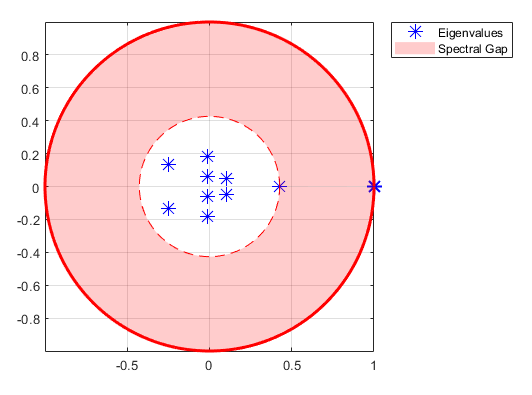
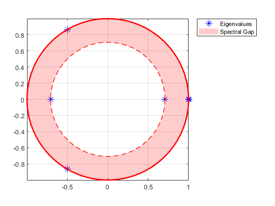
π0. The asymptotics object function computes , if it exists, and estimates the mixing time using eigenvalue
analysis. The eigplot
object function plots the eigenvalues of P. This figure shows an
example of an eigenvalue plot returned by eigplot.
One obstacle to convergence is periodicity. The lazy
object function eliminates periodicity by adjusting state inertia (that is, by
weighting the diagonal elements of P) to produce specified
amounts of “laziness” in the chain. Limiting distributions are unaffected by these
transformations.
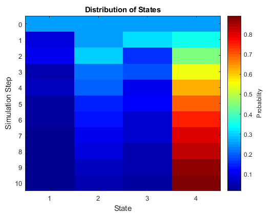
The simulate
and redistribute object functions provide realizations of the process as
it evolves from a specified initial state or distribution. The simplot
and distplot
object functions provide various visualizations. This figure is an example of a
distribution plot showing the evolution of the state distribution starting from a
uniform initial state distribution.
Markov Chain Analysis Workflow
You can start building a Markov chain model object in two ways:
Identify pertinent discrete states in a process, and then estimate transition probabilities among them. In the simplest case, theory suggests chain structure and the transition matrix P. In this situation, you are interested primarily in how the theory plays out in practice—something that is not always obvious from theory. Once you know P, create a Markov chain object by passing P to
dtmc, which implements a theoretical chain.If you have less specific information on a process, then you must experiment with various numbers of states and feasible transition patterns to reproduce empirical results. The
mcmixfunction provides insight into the skeletal structure of a chain, which can capture essential features in the data. Through an iterative process, you can adjust the randomly generated transition matrix P to suit modeling goals.
For an econometric model builder, the most important consequence of the choice of
P is the asymptotic behavior of the chain. To understand this
behavior, identify and separate the transient states (those states whose return-time
probabilities go to zero asymptotically) from the recurrent states (those states
whose return-time probabilities go to one asymptotically). Transience and recurrence
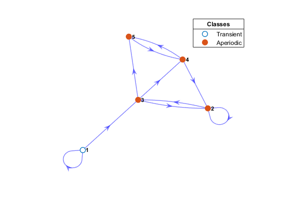
are properties shared by all states in a communicating class. To determine visually
whether states are transient or recurrent, pass the Markov chain object to the
graphplot object function and specify
'ColorNodes',true. Alternatively, the outputs of the
classify
object function provide numerical tools for evaluation. This figure is an example of
a digraph with classified nodes.
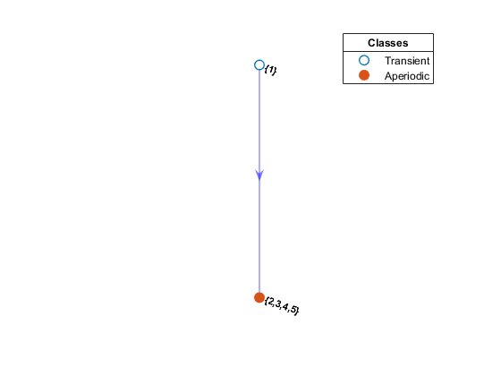
The condensed view of the digraph simplifies this evaluation by consolidating each
communicating class into a “supernode.” In the condensed graph, you can easily
recognize transience and recurrence by the out degree of the supernode (an out
degree greater than 0 implies transience). Irreducible chains
consist of a single, necessarily recurrent, communicating class.
Unichains consist of a single recurrent class and any
number of satellite transient classes. Unichains maintain the desirable limiting
behavior of an irreducible chain. Consideration of the condensed graph is often a
precursor to trimming a chain of irrelevant transient states. The subchain
function trims chains of transient classes. This figure is the condensed view of the
digraph in the previous figure.
The two principle obstacles to uniform limiting behavior are:
Reducibility, the existence of more than one communicating class
Periodicity, the tendency to cycle among subclasses within a single class
A combination of the graphplot and classify
object functions can identify these issues. If a chain is reducible and not a
unichain, it is common to split the analysis among the independent recurrent classes
or reformulate the chain altogether. If a chain is periodic (that is, it contains a
periodic recurrent class), but the overall structure captures the essential details
of an application, the lazy
object function provides a remedy. Lazy chains perturb the diagonal elements of
P to eliminate periodicity, leaving asymptotics
unaffected.
The isreducible and isergodic object functions summarize state classification. Every
chain has a stationary distribution
, where , as a result of P being stochastic and having
an eigenvalue of one. If the chain is irreducible, the stationary distribution is
unique. However, irreducibility, while sufficient, is not a necessary condition for
uniqueness. Unichains also lead to a unique stationary distribution having zero
probability mass in the transient states. In this regard, state classification
analysis is essential because isreducible returns
true only if the chain as a whole consists of a single
communicating class. isreducible returns
false for arbitrary unichains, in which case you must decide
whether transient classes are a relevant part of the model.
Ergodicity, or primitivity, is the
combination of irreducibility and aperiodicity. An ergodic chain has a unique
limiting distribution, that is, π0
converges to for every initial distribution
π0. You can determine whether the
chain, as a whole, is ergodic by using isergodic. The function
identifies ergodic unichains by evaluating the sole recurrent class. A chain is
periodic if it is irreducible and not ergodic, that is, if
~tfirreduc + ~tfergo =
false, where tfirreduc and
tfergo are returned by isreducible and
isergodic, respectively.
Once you have confirmed that a chain is ergodic, you can determine the unique
limiting distribution by using the asymptotics object function. asymptotics returns the limiting distribution and an estimate of the mixing time, which is a time constant for
the decay of transient behavior. The Perron-Frobenius theorem for irreducible
nonnegative matrices (see [1]) is useful for
interpreting these results. Any stochastic matrix has a spectral radius of one.
Periodic matrices, of period k, have k
eigenvalues distributed uniformly around the unit circle at the k
roots of unity. The magnitude of the largest eigenvalue inside the unit circle
determines the decay rate of transient states. The eigplot
object function provides quick visualization of this information. This figure is an
eigenvalue plot of a Markov chain with a period of three.
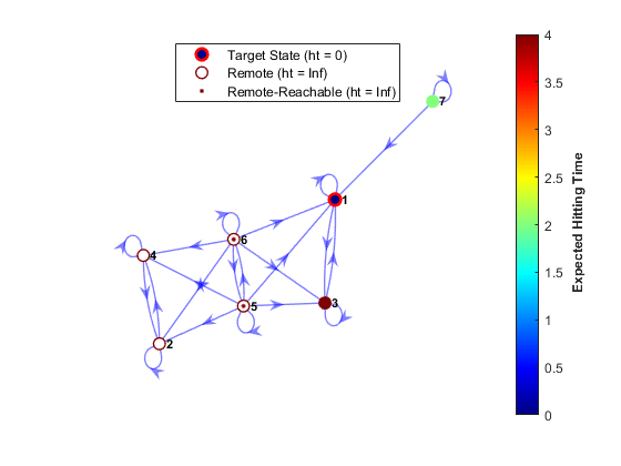
Regardless of the asymptotic properties of the chain, you can study its mixing
rate by applying finite-step analysis. The hitprob
and hittime
functions return hitting probabilities and expected first hitting times for a subset
of target states, beginning from each state in the chain. Both functions optionally
plot a digraph with node colors specifying the hitting probabilities or times. This
figure shows an example of a digraph with node colors specifying the expected first
hitting times. The digraph also indicates whether the beginning states are remote
for the target.
Simulation and redistribution allow you to generate statistical information on the
chain that is difficult to derive directly from the theory. The simulate
and simplot
object functions, and the redistribute and distplot
object functions, provide computational and graphical tools for such analyses.
simulate, for example, generates independent random walks
through the chain. As with simulate and object functions
elsewhere in Econometrics Toolbox™, ensemble averages of dependent statistics play an important role in
forecasting. The corresponding simplot object function offers
several approaches to visualization. This figure displays the proportion of states
visited after 100 random walks of length 10 steps through the periodic Markov chain
in the previous figure.

References
[1] Horn, R., and C. R. Johnson. Matrix Analysis. Cambridge, UK: Cambridge University Press, 1985.
See Also
Objects
Functions
mcmix|graphplot|condensation|bfsearch