Design Optimization Using AI Model
R2026bThis example shows how to speed up a design optimization by using an AI-based surrogate model. The workflow includes:
A computationally expensive design with a response variable of interest
Design of experiments (DOE) to generate predictor data points and evaluate the response data
Training the AI model on the predictor and response data
Performing optimization with the AI model
Post-optimization analysis to understand the results
The approach is to train an AI model to approximate a computationally expensive design, such as a finite-element simulation or a physical experiment. A trained model can make predictions efficiently. This approach enables rapid design space exploration, including relatively fast optimization to identify designs that meet specified objectives and constraints.
This example is an adaptation of Design Optimization for Reaching Target Temperature (Partial Differential Equation Toolbox). The problem is to design a heated block that is cooled using pipes carrying water. The problem uses the Partial Differential Equation Toolbox™ to compute the temperature distribution using finite elements, Statistics and Machine Learning Toolbox™ to design experiments and train an AI-based surrogate model, and the Global Optimization Toolbox to optimize the resulting surrogate model.
Design Problem
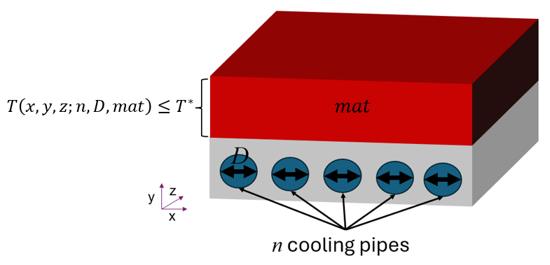
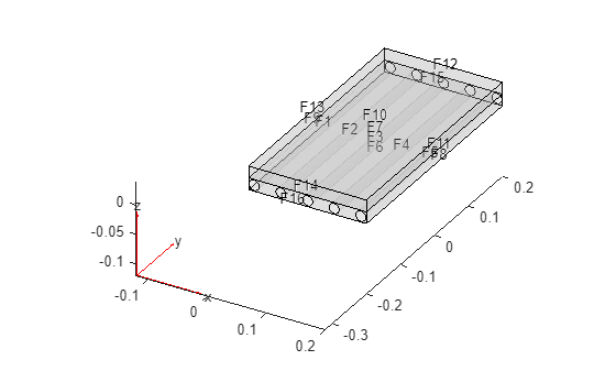
The problem is to optimize the number of cooling pipes , the diameters of the pipes , and the top block material mat to ensure the top block reaches, but does not exceed, a target temperature of . All pipes have the same diameter. The design is subject to these constraints:
The number of pipes is an integer from 1 through 9:
The pipe diameters are continuous from 0.005 through 0.019:
The top block material is aluminum, steel, or iron:
Define Variables
Define the design variables.
variableNames = ["numPipes" "pipeDiam" "blockMaterial"];
nvars = numel(variableNames);
numPipesSet = 1:9;
pipeDiamLimits = [0.005 0.019];
blockMaterialSet = ["aluminum" "steel" "iron"];
Tstar = 385.15;
Evaluate Design
To calculate the maximum temperature in the top block, use Partial Differential Equation Toolbox functions. The calcMaxTemperature helper function at the end of this example calculates the maximum temperature using functions from this toolbox.
Evaluate the design at a sample point to ensure that calcMaxTemperature runs without error. Check the time required for this calculation to determine if calcMaxTemperature is a time-consuming function.
numPipesSample = 5;
pipeDiamSample = 0.01;
blockMaterialSample = "steel";
tic
temperatureSample = calcMaxTemperature(numPipesSample,pipeDiamSample,blockMaterialSample)
temperatureSample = 391.7265
timeToCalculate = toc
timeToCalculate =
10.6743
The calculation time is on the order of 10 seconds.
Design of Experiments
Create data for training an AI model to approximate the underlying finite-element calculation.
Generate Predictor Data Points
Create space-filling predictor data points for the design variables. Determining the number of points to use is often an iterative process. For this example, use 100 points. See Generating Quasi-Random Numbers (Statistics and Machine Learning Toolbox) for more information on space-filling experimental designs.
rng("default")
numPoints = 100;
p = sobolset(nvars);
ps = scramble(p,"MatousekAffineOwen");
q = qrandstream(ps);
pts = qrand(q,numPoints);
The sobolset function returns values between 0 and 1. Map the values to the expected ranges of the design variables. For integer and categorical variables, mapping involves binning or grouping each point into a member of the set.
numPipesBinEdges = linspace(0,1,numel(numPipesSet)+1);
numPipesPredictor = discretize(pts(:,1),numPipesBinEdges,numPipesSet);
pipeDiamPredictor = rescale(pts(:,2),pipeDiamLimits(1),pipeDiamLimits(2));
blockMaterialBinEdges = linspace(0,1,numel(blockMaterialSet)+1);
blockMaterialPredictor = discretize(pts(:,3),blockMaterialBinEdges,blockMaterialSet);
Create a table from the predictor data.
trainingData = table(numPipesPredictor,pipeDiamPredictor,blockMaterialPredictor,VariableNames=variableNames);
Calculate Response Data
Calculate the temperature response data at each point and add the data to the table. Because the finite-element calculations are time consuming, use the training data in the TrainingData.mat file included with this example. The commented code shows how to create the training data on your own.
% temperatureResponse = nan(height(trainingData),1);
% parfor ct = 1:numel(temperatureResponse) % Replace "parfor" with "for" if not using Parallel Computing Toolbox™
%     thisPoint = table2cell(trainingData(ct,:));
%     temperatureResponse(ct) = calcMaxTemperature(thisPoint{:});
% end
% trainingData = addvars(trainingData,temperatureResponse,NewVariableNames="temperature");
load("TrainingData.mat","trainingData");
Visualize Data
Visualize the training data. The plotDesignData helper function at the end of this example uses bubblechart to display the training data and yline to display the target temperature of the design. The maximum temperature of the block generally decreases as the number of pipes increases. For a given number of pipes, the temperature generally decreases as the pipe diameter increases.
plotDesignData(trainingData,Tstar,"Training Data");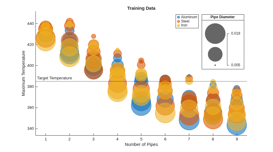
Train AI Model
Train a regression model to approximate the underlying finite-element simulation.
Regression Learner
The Regression Learner (Statistics and Machine Learning Toolbox) app is an interactive tool you can use to train regression models to predict data. You can use the app to automatically train all model types. You can also export a function from the app for training the best performing model, based on the validation root mean square error (RMSE). The trainRegressionModel helper function at the end of this example provides the exported function for this example.
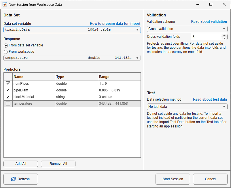
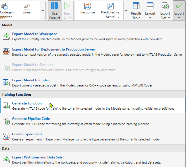
Train Regression Model
The trainRegressionModel helper function trains a Gaussian process regression model, which is commonly used as a surrogate model for expensive physics-based simulations. The function returns a struct that includes the underlying regression model and various other fields with information about the trained model.
trainedModel = trainRegressionModel(trainingData);
The trained model is an approximation (surrogate) of the underlying finite-element simulation. Before exporting a function from Regression Learner, you can perform further testing, as shown in the example Check Model Performance Using Test Data Set in Regression Learner App (Statistics and Machine Learning Toolbox). You can also interpret the model performance, as shown in the example Explain Model Predictions for Regression Models Trained in Regression Learner App (Statistics and Machine Learning Toolbox). Finally, you can consider using features to improve the model, as shown in the example Compare and Improve Regression Models (Statistics and Machine Learning Toolbox).
Predict Values for New Data
Use live controls and the trained model to interactively predict maximum temperature values for new design variables. The predictions are fast compared to the finite-element calculations, as you can see by timing a prediction using tic and toc.
numPipesExplore =numPipesSet(4); pipeDiamExplore =
0.012965; blockMaterialExplore =
blockMaterialSet(1); tic temperaturePredicted = trainedModel.predictFcn(table(numPipesExplore,pipeDiamExplore,blockMaterialExplore,VariableNames=variableNames))
temperaturePredicted =
390.9027
timeToPredict = toc
timeToPredict =
0.0573
speedupFactor = timeToCalculate/timeToPredict
speedupFactor =
186.2594
Solve Optimization Problem
Define and solve an optimization problem using the trained model to predict the maximum temperature.
Formulate the optimization problem using the Problem-Based Optimization Workflow, which provides an easy-to-use interface. First, define the optimization variables. Then, define the problem objective and constraints as expressions of those variables.
Define Optimization Variables
Define the optimization variables using the optimvar function. Include the variable type (integer or continuous) and bounds. Model the nominal categorical variable blockMaterial by using Dummy Variables (Statistics and Machine Learning Toolbox), which are logical variables indicating the block material used. For example, if both the isAluminum and IsSteel binary variables are false, then the material must be iron. The dummyvars2material helper function at the end of this example converts the dummy variables to the material name.
numPipes = optimvar("numPipes",Type="integer",LowerBound=numPipesSet(1),UpperBound=numPipesSet(end));
pipeDiam = optimvar("pipeDiam",LowerBound=pipeDiamLimits(1),UpperBound=pipeDiamLimits(2));
isAluminum = optimvar("isAluminum",Type="integer",LowerBound=0,UpperBound=1);
isSteel = optimvar("isSteel",Type="integer",LowerBound=0,UpperBound=1);
Define Expression to Return Predicted Temperature
Define an expression of the optimization variables that returns the predicted maximum temperature from the trained model. Because the temperature prediction requires unsupported operations on optimization variables (see Supported Operations for Optimization Variables and Expressions), use the fcn2optimexpr function to convert the predictMaxTemperature function to an optimization expression.
temperature = fcn2optimexpr(@predictMaxTemperature,trainedModel,numPipes,pipeDiam,isAluminum,isSteel);
The optimization variables passed to the predictMaxTemperature function must be mapped to the form expected by the trained model's predict function. In this case, the predict function accepts a table with the required variable names.
function temperature = predictMaxTemperature(trainedModel,numPipes,pipeDiam,isAluminum,isSteel)

% Convert the optimization variables to a table.
blockMaterial = dummyvars2material(isAluminum,isSteel);
data = table(numPipes,pipeDiam,blockMaterial,VariableNames=trainedModel.RequiredVariables);

% Return the predicted temperature from the trained model.
temperature = trainedModel.predictFcn(data);
end
Define Objective Function
The objective is the squared difference between the maximum temperature and the target temperature.
Create an optimization problem that includes this objective function. The problem is to minimize this objective function.
problem = optimproblem(Objective=(Tstar-temperature)^2,ObjectiveSense="minimize");Add Constraints
Add problem constraints to ensure that the block is a single material and that its maximum temperature does not exceed the threshold.
problem.Constraints.mustBeOneMaterial = isAluminum + isSteel <= 1;
problem.Constraints.mustNotExceedTempThreshold = temperature <= Tstar;
Review Problem
Display information about the problem formulation.
show(problem)
  OptimizationProblem :

	Solve for:
       isAluminum, isSteel, numPipes, pipeDiam
	where:
       isAluminum, isSteel, numPipes integer
	minimize :
       (385.15 - arg1).^2

       where:

           arg1 = predictMaxTemperature(extraParams{1}, numPipes, pipeDiam, isAluminum, isSteel);

       extraParams


	subject to mustBeOneMaterial:
       isAluminum + isSteel <= 1

	subject to mustNotExceedTempThreshold:
       arg_LHS <= 385.15

       where:

             arg1 = predictMaxTemperature(extraParams{1}, numPipes, pipeDiam, isAluminum, isSteel);
             arg_LHS = arg1;

       extraParams

	variable bounds:
       0 <= isAluminum <= 1

       0 <= isSteel <= 1

       1 <= numPipes <= 9

       0.005 <= pipeDiam <= 0.019
Solve Problem
Solve the problem using the default solver (ga).
rng("default")
[solution,objectiveValue,exitFlag,output] = solve(problem)
Solving problem using ga. ga stopped because the average change in the penalty function value is less than options.FunctionTolerance and the constraint violation is less than options.ConstraintTolerance.
solution = struct with fields:
    isAluminum: 0
       isSteel: 0
      numPipes: 6
      pipeDiam: 0.0091
objectiveValue =
1.1069e-13
exitFlag =
    SolverConvergedSuccessfully
output = struct with fields:
      problemtype: 'integerconstraints'
         rngstate: [1×1 struct]
      generations: 75
        funccount: 2893
          message: 'ga stopped because the average change in the penalty function value is less than options.FunctionTolerance and ↵the constraint violation is less than options.ConstraintTolerance.'
    maxconstraint: 0
       hybridflag: []
           solver: 'ga'
Convert the isAluminum and IsSteel binary variables to the block material name.
blockMaterial = dummyvars2material(solution.isAluminum,solution.isSteel)
blockMaterial =
"iron"
Post-Optimization Analysis
Validate and visualize the optimized design.
Because the trained model is an approximation of the finite-element model, the returned optimized solution can differ from the true optimal value. To compute the actual maximum temperature of the optimized design, rerun the finite-element calculation on the returned solution.
[actual,results] = calcMaxTemperature(solution.numPipes,solution.pipeDiam,blockMaterial);
Calculate the absolute percentage error between the actual and predicted maximum temperatures for the optimized design. If you are not satisfied with the result, you can consider revisiting the Design of Experiments and Train AI Model sections to improve the model performance. You can also try using sobolset again to increase the sampling resolution by adding predictor and response data to the existing set.
predicted = evaluate(temperature,solution);
percentError = mape(predicted,actual)
percentError =
0.0372
Check whether the actual maximum temperature is less than the threshold (mustNotExceedTempThreshold optimization problem constraint) within a specified tolerance.
tol = 1e-3;
isSatisified = actual <= Tstar + tol
isSatisified = logical
   1
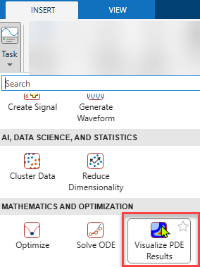
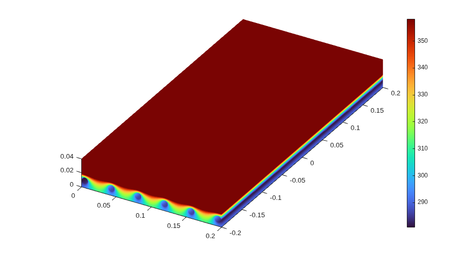
Plot the optimal temperature distribution using the Visualize PDE Results Live Editor task. Usually, you place the task into the script by selecting Task > Visualize PDE Results on the Live Editor tab, or by selecting Task > Visualize PDE Results on the Insert tab.
Plot the temperature distribution by selecting the results object and specifying the Temperature data parameter.
% Data to visualize
meshData = results.Mesh;
nodalData = results.Temperature;

% Create PDE result visualization
resultViz = pdeviz(meshData,nodalData, ...
    "ColorLimits",[280.9 358.2]);
% Clear temporary variables
clearvars meshData nodalData
Conclusion
AI-based surrogate models can be trained to approximate expensive (time-consuming) calculations, such as finite-element simulations. Although AI models take time to train, you can then use them to make predictions for new design variables with a significant speedup factor compared to the original design. This process can accelerate design space exploration, including optimization workflows to identify designs that meet specified objectives and constraints. However, because the resulting model is an approximation of the underlying design, you must investigate the optimized solution to understand the result.
Helper Functions
The calcMaxTemperature function accepts the design variables and returns the maximum temperature in the top block geometry.
function [temperature,resultsObj] = calcMaxTemperature(numPipes,pipeDiam,blockMaterial)

% Specify the length, width, and height of the cooling plate.
% The top block has the same parameters.
L = 0.4; % length in meters
W = 0.2; % width in meters
H = 0.02; % height same as height of the top block

% Specify the gap between the edge of the plate and a pipe.
edgeGap = 1.1*pipeDiam/2; % in meters

% Create the stacked cuboids geometry representing the block and the
% cooling plate.
g = multicuboid(W,L,[H H],ZOffset=[0 H]);
g = fegeometry(translate(g,[W/2,0,0]));

% Create the geometry representing a pipe.
gCyl = fegeometry(multicylinder(pipeDiam/2,L));
gCyl = rotate(gCyl,90,[0 0 0],[1 0 0]);

% Combine the geometries to represent the top block and the
% cooling plate with the pipes.
if numPipes == 1
    gCylT = translate(gCyl,[W/2,L/2,H/2]);
    g = subtract(g,gCylT);
else
    gPipes = fegeometry;
    for k=linspace(edgeGap,W-edgeGap,numPipes)
        gCylT = translate(gCyl,[k,L/2,H/2]);
        gPipes = union(gPipes,gCylT);
    end
    g=subtract(g,gPipes);
end

% Create an femodel object for thermal steady-state analysis and
% include the geometry in the model.
model = femodel(AnalysisType="thermalSteady", ...
    Geometry=g);

% Specify the thermal conductivity of the cooling plate.
model.MaterialProperties(1) = ...
    materialProperties(ThermalConductivity=0.5);

% Specify the thermal conductivity of the top block, which produces heat.
model.MaterialProperties(2) = ...
    materialProperties(Material=blockMaterial);

% Specify the heat source in the top block.
powerWattage = 0.5E3;
volTopBlock = W*L*H;
heatSource = powerWattage/volTopBlock;
model.CellLoad(2) = cellLoad(Heat=heatSource);

% Compute heat transfer coefficient for the convective boundary condition.
m_dot = 0.02; % Mass flow rate, in kg/s
mu = 0.001002; % Dynamic viscosity of water at 293.15K, in kg/(m*s)
Re = (4*m_dot)/(pi*pipeDiam*mu); % Reynolds number
Pr = 7.2; % Prandtl number of water at 293.15K
if Re >= 10000
    Nu = 0.023*Re^0.8*Pr^0.4; % Nusselt number; use the Dittus-Boelter equation for high Re
else
    Nu = 3.66; % Else assume the Nu constant
end
k = 0.598; % Thermal conductivity of water at 293.15K (W/(m*K))
htc = (Nu*k)/pipeDiam; % Heat transfer coefficient

% Specify natural convection to ambient on all external faces of the top block
% and cooling plate. Here, blockFaces include all faces except the pipes and
% the face between the blocks.
blockFaces = [numPipes+1,(numPipes+3):g.NumFaces];
model.FaceLoad(blockFaces) = faceLoad(ConvectionCoefficient=20, ...
    AmbientTemperature=298.15);

% Specify the forced convection of chilled water in the pipes.
pipeFaces = 1:numPipes;  % Faces corresponding to the pipes
model.FaceLoad(pipeFaces) = faceLoad(ConvectionCoefficient=htc, ...
    AmbientTemperature=278.15);

% Generate a mesh.
model = generateMesh(model,Hface={pipeFaces,pipeDiam/5});

% Solve the model.
resultsObj = solve(model);

% Find the max temperature.
temperature = max(resultsObj.Temperature);
end
The plotDesignData function uses bubblechart to display the data and yline to display the target temperature of the design.
function plotDesignData(data,Tstar,titletext)

% Size the figure for clarity.
f = figure();
width = 900;
height = 500;
f.Position(3:4) = [width,height];

% Plot each material as a bubblechart and the target temperature as a
% horizontal line.
hold on
aluminumInd = strcmp(data.blockMaterial,"aluminum");
steelInd = strcmp(data.blockMaterial,"steel");
ironInd = strcmp(data.blockMaterial,"iron");
bubblechart(data.numPipes(aluminumInd),data.temperature(aluminumInd),data.pipeDiam(aluminumInd));
bubblechart(data.numPipes(steelInd),data.temperature(steelInd),data.pipeDiam(steelInd));
bubblechart(data.numPipes(ironInd),data.temperature(ironInd),data.pipeDiam(ironInd));
yline(Tstar,"-","Target Temperature",LabelHorizontalAlignment="left");
hold off

% Add plot labels
title(titletext)
xlabel("Number of Pipes")
ylabel("Maximum Temperature")
bubblelegend("Pipe Diameter");
legend("Aluminum","Steel","Iron")
end
The trainRegressionModel function trains the best performing regression model based on the validation RMSE found with the Regression Learner app.
function [trainedModel,validationRMSE] = trainRegressionModel(trainingData)
% [trainedModel,validationRMSE] = trainRegressionModel(trainingData)
% Return a trained regression model and its RMSE. This code recreates the
% model trained in the Regression Learner app. Use the generated code to
% automate training the same model with new data, or to learn how to
% programmatically train models.
%
%  Input:
%      trainingData: A table containing the same predictor and response
%       columns as those imported into the app.
%
%
%  Output:
%      trainedModel: A struct containing the trained regression model. The
%       struct contains various fields with information about the trained
%       model.
%
%      trainedModel.predictFcn: A function to make predictions on new data.
%
%      validationRMSE: A double representing the validation RMSE. In the
%       app, the Models pane displays the validation RMSE for each model.
%
% Use the code to train the model with new data. To retrain your model,
% call the function from the command line with your original data or new
% data as the input argument trainingData.
%
% For example, to retrain a regression model trained with the original data
% set T, enter:
%   [trainedModel,validationRMSE] = trainRegressionModel(T)
%
% To make predictions with the returned trainedModel on new data T2, enter:
%   yfit = trainedModel.predictFcn(T2)
%
% T2 must be a table containing at least the same predictor columns as those used
% during training. For details, enter:
%   trainedModel.HowToPredict

% Auto-generated by MATLAB on 03-Mar-2026 14:15:48


% Extract the predictors and response.
% This code processes the data into the right shape for training the
% model.
inputTable = trainingData;
predictorNames = ["numPipes","pipeDiam","blockMaterial"];
predictors = inputTable(:,predictorNames);
response = inputTable.temperature;
isCategoricalPredictor = [false, false, true];

% Train a regression model.
% This code specifies all the model options and trains the model.
regressionGP = fitrgp(...
    predictors, ...
    response, ...
    BasisFunction="constant", ...
    KernelFunction="exponential", ...
    Standardize=true);

% Create the result struct with predict function
predictorExtractionFcn = @(t) t(:, predictorNames);
gpPredictFcn = @(x) predict(regressionGP, x);
trainedModel.predictFcn = @(x) gpPredictFcn(predictorExtractionFcn(x));

% Add additional fields to the result struct
trainedModel.RequiredVariables = ["numPipes","pipeDiam","blockMaterial"];
trainedModel.RegressionGP = regressionGP;
trainedModel.About = "This struct is a trained model exported from Regression Learner R2026a.";
trainedModel.HowToPredict = sprintf('To make predictions on a new table, T, use: \n  yfit = c.predictFcn(T) \nreplace ''c'' with the name of the variable that is this struct, e.g. ''trainedModel''. \n \nThe table, T, must contain the variables returned by: \n  c.RequiredVariables \nVariable formats (e.g. matrix/vector, datatype) must match the original training data. \nAdditional variables are ignored. \n \nFor more information, see <a href="matlab:helpview(fullfile(docroot, ''stats'', ''stats.map''), ''appregression_exportmodeltoworkspace'')">How to predict using an exported model</a>.');

% Extract predictors and response
% This code processes the data into the right shape for training the
% model.
inputTable = trainingData;
predictorNames = ["numPipes","pipeDiam","blockMaterial"];
predictors = inputTable(:, predictorNames);
response = inputTable.temperature;
isCategoricalPredictor = [false, false, true];

% Perform cross-validation
partitionedModel = crossval(trainedModel.RegressionGP,KFold=5);

% Compute validation predictions
validationPredictions = kfoldPredict(partitionedModel);

% Compute validation RMSE
validationRMSE = sqrt(kfoldLoss(partitionedModel,LossFun="mse"));
end
The dummyvars2material function converts the dummy variables isAluminum and isSteel to the top block material name.
function material = dummyvars2material(isAluminum,isSteel)
% Convert dummy variables to material name.

if isAluminum
    material = "aluminum";
elseif isSteel
    material = "steel";
else
    material = "iron";
end
end
See Also
Topics
- Design Optimization for Reaching Target Temperature (Partial Differential Equation Toolbox)
- Regression Learner (Statistics and Machine Learning Toolbox)
- Problem-Based Optimization Workflow

