Compare No Reference Image Quality Metrics
This example shows how to compare the performance of various blind or no-reference image quality metrics.
Evaluating the quality of an image is an important part of image acquisition, compression, and other image enhancement workflows. It is desirable to have a fast, automated metric that closely mimics subjective measures of image quality. This example compares the performance of three no-reference quality metrics.
BRISQUE - Blind/Referenceless image spatial quality evaluator
NIQE - Naturalness image quality evaluator
PIQE - Perception-based image quality evaluator
Each metric has different strengths depending on the images in the data set. To select the best metric for your data, you can compare the performance of the three metrics on sample image data. This example shows how to compare the performance in two different situations: varying levels of JPEG compression on a single image and for a video stream.
Evaluate Response to Varying Compression on Single Image
Image compression is a tradeoff between visual quality and the compression ratio, or size of the output data. The tradeoff also depends on the image content. For example, images with uniform areas can compress to smaller file sizes and exhibit fewer artifacts than images with detailed features. Image quality metrics can help analyze this tradeoff, while trying to minimize the impact of the image content on the analysis.
Read an image into the workspace.
im = imread('llama.jpg');Write copies of the image with different JPG compression ratios. Read each compressed image back into the workspace.
jpegQuality = 10:10:100;
numObservations = numel(jpegQuality);
compressedFrames = cell(1,numObservations);
for ind = 1:numObservations
    q = jpegQuality(ind);
    tempFile = ['llama_compression_',num2str(q),'.jpg'];
    imwrite(im,tempFile,'Quality',q);
    compressedFrames{ind} = imread(tempFile);
end
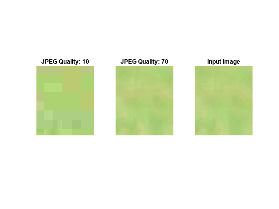
Inspect the compressed images.
tiledlayout(1,3);

h1 = nexttile;
imshow(compressedFrames{1})
title('JPEG Quality: 10')

nexttile
imshow(compressedFrames{7})
title('JPEG Quality: 70')

nexttile
imshow(im)
title('Input Image')
linkaxes
Zoom in on the compressed image to see the nature of some specific artifacts. At JPEG quality 10, the blocking artifacts are obvious.
h1.XLim = [650 700];
h1.YLim = [490 550];
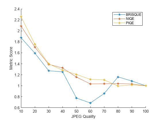
For each compressed JPG image, calculate the quality score using the three quality metrics.
pQ = zeros(1, numObservations);
nQ = zeros(1, numObservations);
bQ = zeros(1, numObservations);

for ind=1:numObservations
    bQ(ind) = brisque(compressedFrames{ind});
    nQ(ind) = niqe(compressedFrames{ind});
    pQ(ind) = piqe(compressedFrames{ind});
end
Visualize the score of the metrics as the JPEG quality increases. Normalize the scores so that each score has the same value for the uncompressed image. For these three metrics, lower scores correspond to higher image quality.
The BRISQUE score for a JPEG quality of 50, 60, and 70 is unrealistically lower than for uncompressed JPEG images. Therefore, for images similar to this test image, NIQE and PIQE are more reliable metrics.
figure
hold on
plot(jpegQuality,bQ/bQ(end),'*-');
plot(jpegQuality,nQ/nQ(end),'*-');
plot(jpegQuality,pQ/pQ(end),'*-');
legend('BRISQUE','NIQE','PIQE');
ylabel('Metric Score')
xlabel('JPEG Quality')
hold off
Evaluate Response to Varying Compression and Content Using a Video
In applications such as streaming video, there is a need to evaluate quality metrics at the receiver which may not have access to the original pristine sample. Also, the content of each frame can vary significantly. Let us simulate such a scenario to evaluate the performance characteristics of these metrics.
Create a VideoReader object that reads frames from the video 'rhinos.avi'. This video has 114 frames.
vidObjR = VideoReader('rhinos.avi');
vidObjW = VideoWriter('varyingCompressed.avi');
open(vidObjW)
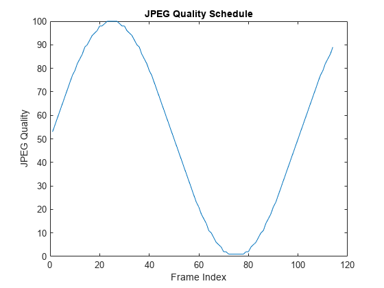
Create a varying compression ratio schedule to mimic real time varying bitrate transmissions.
numFrames = vidObjR.NumFrames;
varyingQuality = sin(2*pi*(1:numFrames)*0.01);
varyingQuality = round(rescale(varyingQuality)*100);
varyingQuality = max(varyingQuality,1); % min JPEG quality is 1

figure
plot(varyingQuality);
title('JPEG Quality Schedule');
ylabel('JPEG Quality')
xlabel('Frame Index')
For each frame in the video, compress the frame according to the JPEG quality schedule. Compute the metrics of the compressed frame and add the compressed frame to the output video for validation.
pQ = zeros(1,numFrames);
nQ = zeros(1,numFrames);
bQ = zeros(1,numFrames);

ind = 1;
while hasFrame(vidObjR)
    im = readFrame(vidObjR);

    % Compress it based on the schedule
    tempFile = 'rhinos_compressed_frame.jpg';
    imwrite(im,tempFile,'Quality',varyingQuality(ind));
    frame = imread(tempFile);

    writeVideo(vidObjW,frame);

    bQ(ind) = brisque(frame);
    nQ(ind) = niqe(frame);
    pQ(ind) = piqe(frame);
    ind = ind+1;
end
close(vidObjW);
Visualize the trend, expect it to mimic the compression schedule. Rescale the metrics to focus on the trend, and invert the quality schedule to get the compression ratio trend. Quality metrics can still give a useful indication of perceived quality without access to the original reference frame.
figure
hold on
plot(rescale(bQ));
plot(rescale(nQ));
plot(rescale(pQ));
% Invert JPEG Quality to get the compression ratio
plot(1-rescale(varyingQuality),'k','LineWidth',2)
legend('BRISQUE','NIQE','PIQE','Compression Ratio');
title('Trend of Quality Metrics with Varying Compression and Content');
ylabel('Metric Score')
xlabel('Frame Index')
hold off

See Also
fitbrisque | brisqueModel | niqe | niqeModel | fitniqe | brisque