Find Drive Characteristics and Generate Optimal Reference Current LUTs
Define Speed and Torque Grid
After you compute surface maps (as mentioned in the previous step), you can define the speed and torque breakpoints over which to generate the reference id and iq current LUTs. The maximum speed and torque values cover the maximum values achievable in this example PMSM application.
The script DriveCharacteristicsCurrentLUTs.m contains the code to
find drive characteristics and generate optimal reference current LUTs. To open this script,
run this command:
openExample("DriveCharacteristicsCurrentLUTs.m")In the first code section, adjust these values to suit the range of speeds and torques appropriate for your motor setup and simulation needs. Additionally, adjust the number of grid points ngridpts along each dimension. More grid points improves the accuracy of nonlinearity tracing for LUT generation, but incurs more costs in terms of memory and computation speed.
pmsm.Rs=Rs;
pmsm.p=pp;
pmsm.I_rated=I_rated;
pmsm.B=1e-6;
pmsm.J=1e-6;
pmsm.T_rated=mcb.PMSMRatedTorque(pmsm,inverter);

ngridpts = 40;
RPMGrid = [100 linspace( 500, min(25000,mcb.PMSMMaxSpeed(pmsm,inverter)), ngridpts)];
TrqMax = max(abs(torque),[],"all");
NmGrid  = [0 0.1 linspace(0.5,min(TrqMax,mcb.PMSMRatedTorque(pmsm,inverter)), ngridpts)];
Load Motor Parameters
Use the second code section in DriveCharacteristicsCurrentLUTs.m to
load the motor parameters into the pmsm and inverter
data
structures.
[id_m1,iq_m1]=meshgrid(idAxis,iqAxis);
pmsm.PMSMLUT.LdTable = interp2(pmsm.PMSMLUT.idVec,pmsm.PMSMLUT.iqVec,pmsm.PMSMLUT.LdTable,IDgrid,IQgrid);
pmsm.PMSMLUT.LqTable = interp2(pmsm.PMSMLUT.idVec,pmsm.PMSMLUT.iqVec,pmsm.PMSMLUT.LqTable,IDgrid,IQgrid);
pmsm.PMSMLUT.FluxPMTable = interp2(pmsm.PMSMLUT.idVec,pmsm.PMSMLUT.iqVec,pmsm.PMSMLUT.FluxPMTable,IDgrid,IQgrid);
pmsm.PMSMLUT.idVec=idAxis;
pmsm.PMSMLUT.iqVec=iqAxis;
pmsm.PMSMLUT.FluxDTable=lambdad;
pmsm.PMSMLUT.FluxQTable=lambdaq;
pmsm.PMSMLUT.method='FluxDQ';
pmsm.PMSMLUT.TorqueTable=torque;
pmsm.PMSMLUT.wrpmVec=double(RPMGrid);
pmsm.PMSMLUT.trefVec=NmGrid;
pmsm.PMSMLUT.motorType='ipmsm';
pmsm.motorType='ipmsm';
inverter.V_dc=Vdc;
Plot Constraint Curves and Drive Characteristics
Determine PMSM constraint curves from the processed data, and plot the associated drive characteristics. For more information about synchronous motor constraint curves and drive characteristics, see these topics:
In the third code section in DriveCharacteristicsCurrentLUTs.m, you
use mcb.PMSMCharacteristics utility to plot the
characteristics.
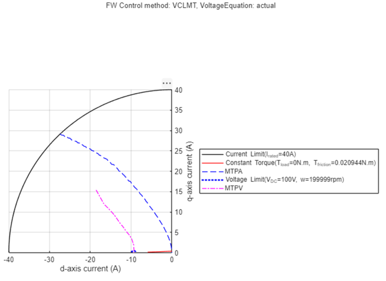
mcb.PMSMCharacteristics(pmsm,inverter,constraintCurves=1);
legend('Location','eastoutside');
In the generated figure as shown below, observe the different constraints of the PMSM, such as current limit curve, voltage limit curve, constant torque curve, MTPA curve and MTPV curve.
Compute and Plot Optimal Reference Currents
Compute optimal reference current LUTs PMSMLUT.idTable and
PMSMLUT.iqTable, then create surface maps of these currents. For more
information about the generation of optimal reference currents, see Plot Constraint Curves and Drive Characteristics for PMSM and SynRM Directly from Block Parameters Dialog Box.
Run the code in the fourth code section in
DriveCharacteristicsCurrentLUTs.m.
PMSMLUT1=PMSMLUT;PMSMLUT=mcb.generateMotorLUT(pmsm,inverter,'idiqluts',useTorquePercent=0,drawLUT=1);In the generated figure as shown below, observe the look-up tables of reference currents plotted in the id-iq plane. Every black dot corresponds to a computed optimal reference current pair at the chosen operating speed and load toque.

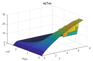
Generate surface curves for id and iq.
figure;surf(PMSMLUT.trefVec,PMSMLUT.wrpmVec,PMSMLUT.idTable');xlabel('T');ylabel('w_{rpm}');title('id(T,w)');

figure;surf(PMSMLUT.trefVec,PMSMLUT.wrpmVec,PMSMLUT.iqTable');xlabel('T');ylabel('w_{rpm}');title('iq(T,w)');