Descripción general de la simulación GNSS
La simulación del Sistema Global de Navegación por Satélite (GNSS) genera estimaciones de la posición del receptor. Estas estimaciones de posición del receptor provienen de modelos de sensores GPS y GNSS como objetos gpsSensor y gnssSensor. Supervise el estado de la estimación de posición en gnssSensor utilizando la dilución de salidas de precisión y compare el número de satélites disponibles.
Parámetros de simulación
Especifique los parámetros que se utilizarán en la simulación GNSS:
Frecuencia de muestreo del receptor GNSS
Sistema de referencia de navegación local
Ubicación en la Tierra en coordenadas de latitud, longitud y altitud (LLA)
Número de muestras a simular
Fs = 1;
refFrame = "NED";
lla0 = [42.2825 -71.343 53.0352];
N = 100;
Cree una trayectoria para un sensor estacionario.
pos = zeros(N,3);
vel = zeros(N,3);
time = (0:N-1)./Fs;
Creación de modelos de sensores
Cree los objetos de simulación GNSS, gpsSensor y gnssSensor, utilizando los mismos parámetros iniciales para cada uno.
gps = gpsSensor(SampleRate=Fs,ReferenceLocation=lla0, ...
    ReferenceFrame=refFrame);

gnss = gnssSensor(SampleRate=Fs,ReferenceLocation=lla0, ...
    ReferenceFrame=refFrame);
Simulación usando gpsSensor
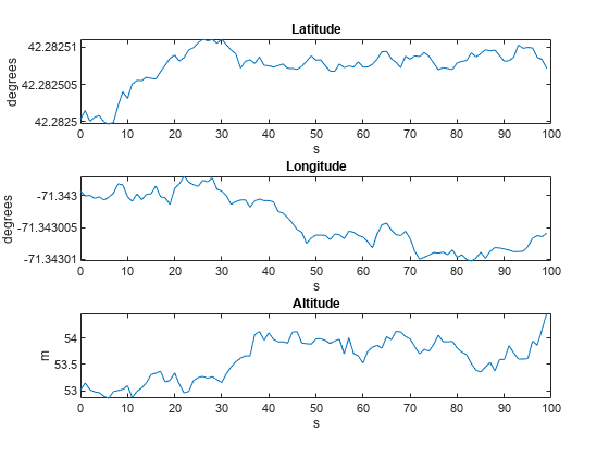
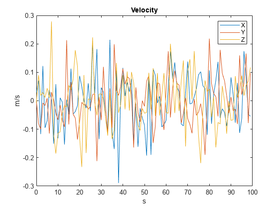
Genere salidas desde un receptor estacionario utilizando el sensor GPS. Visualice la posición en coordenadas LLA y la velocidad en cada dirección.
% Generate outputs.
[llaGPS,velGPS] = gps(pos,vel);

% Visualize position.
figure
subplot(3,1,1)
plot(time,llaGPS(:,1))
title("Latitude")
ylabel("degrees")
xlabel("s")
subplot(3,1,2)
plot(time,llaGPS(:,2))
title("Longitude")
ylabel("degrees")
xlabel("s")
subplot(3,1,3)
plot(time,llaGPS(:,3))
title("Altitude")
ylabel("m")
xlabel('s')
% Visualize velocity.
figure
plot(time,velGPS)
title("Velocity")
legend("X","Y","Z")
ylabel("m/s")
xlabel("s")
Simulación usando gnssSensor
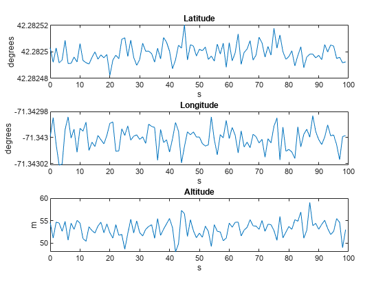
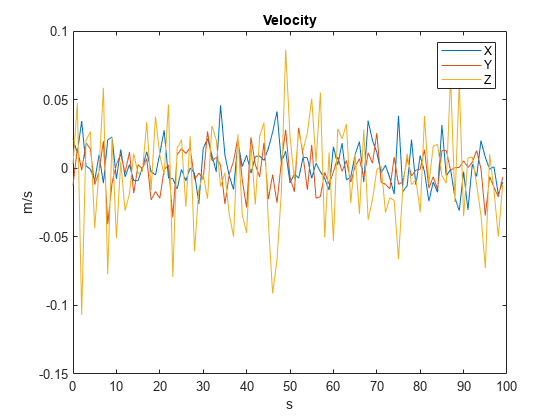
Genere salidas desde un receptor estacionario utilizando el sensor GNSS. Visualice la posición y la velocidad y observe las diferencias en la simulación.
% Generate outputs.
[llaGNSS,velGNSS] = gnss(pos,vel);

% Visualize position.
figure
subplot(3,1,1)
plot(time,llaGNSS(:,1))
title("Latitude")
ylabel("degrees")
xlabel("s")
subplot(3,1,2)
plot(time,llaGNSS(:,2))
title("Longitude")
ylabel("degrees")
xlabel("s")
subplot(3,1,3)
plot(time,llaGNSS(:,3))
title("Altitude")
ylabel("m")
xlabel("s")
% Visualize velocity.
figure
plot(time,velGNSS)
title("Velocity")
legend("X","Y","Z")
ylabel("m/s")
xlabel("s")
Dilución de la precisión
El objeto gnssSensor tiene una simulación de mayor fidelidad en comparación con gpsSensor. Por ejemplo, el objeto gnssSensor utiliza posiciones de satélite simuladas para estimar la posición del receptor. Esto significa que la dilución de precisión horizontal (HDOP) y la dilución de precisión vertical (VDOP) se pueden informar junto con la estimación de posición. Estos valores indican qué tan precisa es la estimación de la posición basada en la geometría del satélite. Los valores más pequeños indican una estimación más precisa.
% Set the RNG seed to reproduce results.
rng("default")

% Specify the start time of the simulation.
initTime = datetime(2020,4,20,18,10,0,TimeZone="America/New_York");

% Create the GNSS receiver model.
gnss = gnssSensor(SampleRate=Fs,ReferenceLocation=lla0, ...
    ReferenceFrame=refFrame,InitialTime=initTime);

% Obtain the receiver status.
[~,~,status] = gnss(pos,vel);
disp(status(1))
      SatelliteAzimuth: [7×1 double]
    SatelliteElevation: [7×1 double]
                  HDOP: 1.1290
                  VDOP: 1.9035
Vea el HDOP durante toda la simulación. Hay una disminución en el HDOP. Esto significa que la geometría del satélite cambió.
hdops = vertcat(status.HDOP);

figure
plot(time,vertcat(status.HDOP))
title("HDOP")
ylabel("m")
xlabel("s")
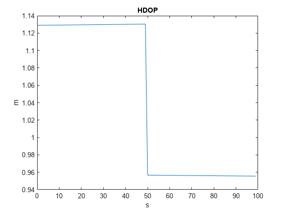
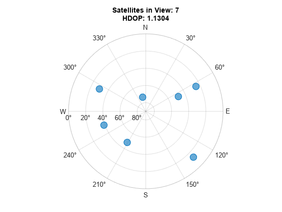
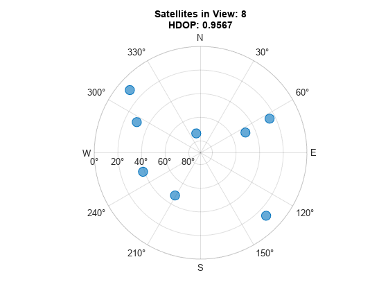
Verifique que la geometría del satélite haya cambiado. Encuentre el índice donde disminuyó el HDOP y vea si eso corresponde a un cambio en la cantidad de satélites a la vista. La variable numSats aumenta de 7 a 8.
% Find expected sample index for a change in the
% number of satellites in view.
[~,satChangeIdx] = max(abs(diff(hdops)));

% Visualize the satellite geometry before the
% change in HDOP.
satAz = status(satChangeIdx).SatelliteAzimuth;
satEl = status(satChangeIdx).SatelliteElevation;
numSats = numel(satAz);
skyplot(satAz,satEl);
title(sprintf('Satellites in View: %d\nHDOP: %.4f', ...
    numSats,hdops(satChangeIdx)))
% Visualize the satellite geometry after the
% change in HDOP.
satAz = status(satChangeIdx+1).SatelliteAzimuth;
satEl = status(satChangeIdx+1).SatelliteElevation;
numSats = numel(satAz);
skyplot(satAz, satEl);
title(sprintf('Satellites in View: %d\nHDOP: %.4f', ...
    numSats,hdops(satChangeIdx+1)))
Los valores HDOP y VDOP se pueden utilizar como elementos diagonales en matrices de covarianza de medición al combinar estimaciones de posición del receptor GNSS con otras mediciones de sensores utilizando un filtro de Kalman.
% Convert HDOP and VDOP to a measurement covariance matrix.
hdop = status(1).HDOP;
vdop = status(1).VDOP;
measCov = diag([hdop.^2/2, hdop.^2/2, vdop.^2]);
disp(measCov)
0.6373 0 0
0 0.6373 0
0 0 3.6233