Sensor Array Analyzer
Analyze beam patterns and performance characteristics of linear, planar, 3-D, and arbitrary sensor arrays
Description
The Sensor Array Analyzer app enables you to construct and analyze common sensor array configurations. These configurations range from 1-D to 3-D arrays of antennas, sonar transducers, and microphones, and can contain subarrays. After you specify array and sensor parameters, the app displays basic performance characteristics such as array directivity and array dimensions. You can then create various directivity plots and images.
Array Types
You can use this app to show the directivity of these arrays:
2D Arrays
Uniform Linear Array (ULA)
Uniform Rectangular Array (URA)
Uniform Circular Array (UCA)
Uniform Hexagonal Array (UHA)
Circular Planar Array
Concentric Array
3D Arrays
Spherical Array
Cylindrical Array
Arbitrary Array
Subarrays
You can use this app to create and analyze arrays containing subarrays to:
Replicate an array along a spatial grid.
Partition a larger array into subarrays.
Element Types
These elements are available to populate an array:
Non-Polarized Antennas
Cardioid Antenna
Cosine Antenna
Custom Antenna
Gaussian Antenna
Isotropic Antenna
Sinc Antenna
Polarized Antennas
Crossed Dipole Antenna
Custom Antenna
NR Antenna
Short Dipole Antenna
Microphones
Cardioid Microphone
Custom Microphone
Omnidirectional Microphone
Sonar Transducers
Isotropic Hydrophone
Isotropic Projector
Plot Options
The Sensor Array Analyzer app can create these types of plots:
Array Geometry
2-D Array Patterns
3-D Array Pattern
Grating Lobes
Open the Sensor Array Analyzer App
MATLAB® toolstrip: On the Apps tab, under Signal Processing and Communications, click the app icon.
MATLAB command prompt: Enter
sensorArrayAnalyzer.
Examples
This example analyzes a 10-element uniform linear array (ULA) in a sonar application. The array consists of isotropic hydrophones. Design the array for a 10 KHz signal.
A uniform linear array has sensor elements that are equally spaced along a line.
Under the Analyzer tab, in the Array section of the toolstrip, select ULA. In the Element section of the toolstrip, select Hydrophone.
Select the Parameters tab and set the Number of
Elements to 10. Set the
Element Spacing to 0.5
wavelengths.
Design the array for a 10 KHz signal by setting Signal
Frequencies (Hz) to 10000. Then click
the Apply button. You can change many menu items and
apply the changes at any time. The parameters that appear in this tab depend
on your choice of array and element.
When you choose a sonar element, the app automatically sets the signal
propagation speed in water to 1500. You can set the
signal propagation speed to any value by setting the Propagation
Speed (m/s).
Select the Array Geometry tab and use the check boxes to display element normals (Show Normals), element indices (Show Index), and element tapers (Show Tapers).

In the rightmost Array Characteristics panel, you can view the array directivity, half-power beam width (HPBW), first-null beam-width (FNBW), and side lobe level (SLL).
To display a directivity plot, go to the Plots
section of the Analyzer tab. Select
Azimuth Pattern from the 2D
Pattern menu. The azimuth directivity pattern is now
displayed in the center panel of the app. Select the Azimuth
Pattern tab, and set the Coordinate to
Rectangular.

You can see the main lobe of the array directivity function (also called the main beam) at 0° and another main lobe at ±180°. Two main lobes appear because of the cylindrical symmetry of the ULA array.
A beam scanner works by successively pointing the array main lobe in
different directions. In the Steering tab, set
Azimuth Angles (deg) to 30 and
Elevation Angles (deg) to 0.
This steers the main lobe to 30° in azimuth and 0° elevation. 
One disadvantage of a ULA is its large side lobes. An examination of the array directivity shows two side lobes close to each main lobe, each down by about only 13 dB. A strong side lobe inhibits the ability of the array to detect a weaker signal in the presence of a larger nearby signal. By using array tapering, you can reduce the side lobes.
Use the Taper option to specify the array taper as a
Taylor window with Sidelobe
Attenuation set to 30 dB and
nbar set to 4. Click the
Apply button.

This example plots the azimuth response of a four-element ULA partitioned into two two-element ULAs.
Under the Analyzer tab, in the Array section of the toolstrip, select ULA. Create a ULA with default parameters (with the number of elements set to 4 and the element spacing set to 0.5 meters).

Select the Partition button on the
Analyzer. Design the array for a 1 GHz signal by
setting Signal Frequencies (Hz) to
1e9. Then click the Apply
button. You can change many menu items and apply the changes at any time.
The parameters that appear in this tab depend on your choice of array and
element.

The subarray selection menu item should read
[ones(1,2) zeros(1,2); zeros(1,2) ones(1,2)].
Select 2D Pattern in the
Analyzer tab and choose the Azimuth
pattern to visualize the 2-D azimuth pattern in polar
coordinates.

A partitioned array consists of multiple subarrays in which each array element can be assigned to one or more subarrays. After creating the partition array, you can then re-assign elements to different subarrays. For example, create a 4-by-4 uniform rectangular array (URA) containing 16 elements. Selecting the Partition tab converts the URA into a 4-by-4 partitioned array with subarrays indicated by different colors. The partitioning is controlled by the Subarray Selection matrix.
[ ones(1,8) zeros(1,8); zeros(1,8) ones(1,8)]
To re-partition an array, you can edit the Subarray Selection matrix. Select the Define Subarray tab to rearrange the elements belonging to the subarrays.

Selecting the Define Subarray tab brings up the subarray editor.

You can:
Select the pencil icon next to Subarray1 to edit the elements and weights in subarray 1.
Select the pencil icon next to Subarray2 to edit the elements and weights in subarray 2.
Select the green cross icon at the top to create an empty subarray.
Select Subarray 2 to display the element indices belonging to Subarray 2.

Remove element 9 and its weight. Select the green cross add a new subarray, Subarray 3. Then add element 9 to the new subarray.

The new subarray and its added element appears in yellow.
This example shows how to construct a 6-by-6 uniform rectangular array (URA) designed to detect and localize a 100 MHz signal.
Under the Analyzer tab, in the Array section of the toolstrip, select URA. In the Element section of the toolstrip, select Isotropic.
Design the array for a 100 MHz signal by setting Signal
Frequencies to 100e6 and the row and
column Element Spacing to [0.5 0.5]
wavelength.
Select the Parameters tab and set the Size to
[6,6].
From the Taper drop-down, choose Row and
Column. Set Row Taper and
Column Taper to a Taylor window
using default taper parameters. Click the Apply button
to apply the changes. You can change many menu items and apply the changes
at any time. The parameters that appear in this tab depend on your choice of
array and element.
The shape of the array is shown in this figure.

Next, display a 3-D array pattern by selecting 3D Pattern in the Plots section of the Analyzer tab.

A significant performance measure for any array is directivity. You can use the app to examine the effects of tapering on array directivity. Without tapering, the array directivity for this URA is 17.16 dB. With tapering, the array directivity is reduced to 16.03 dBi.
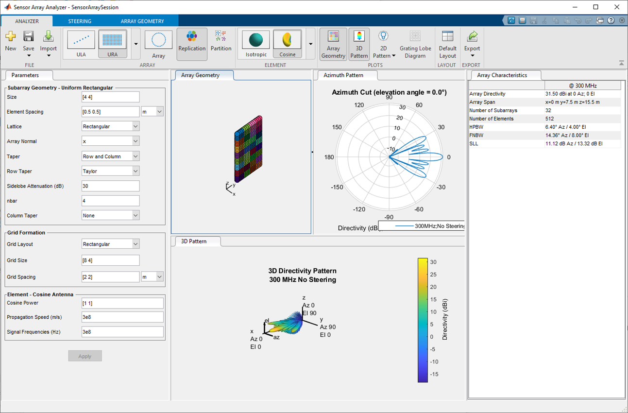
This example shows the grating lobe diagram of a 4-by-4 uniform rectangular array (URA) designed to detect and localize a 300 MHz signal.
Under the Analyzer tab, in the
Array section of the toolstrip, select
URA. In the Element
section of the toolstrip, select Isotropic. Set the
Size to [4,4]. In the
Steering tab, set Azimuth Angles
(deg) to 20 and Elevation Angles
(deg) to 0.
Design the array for a 300 MHz signal by setting Signal
Frequencies to 3e8 and the row and column
Element Spacing to [0.7,0.7]
wavelength. By setting the row and column Element
Spacing to [0.7,0.7] wavelengths, you
create a spatially under-sampled, array. Then click the
Apply button.
Select Grating Lobe Diagram from the Plots section to plot the grating lobes.
This figure shows the grating lobe diagram produced when you beamform the array towards the angle [20,0]. The main lobe is designated by the small black-filled circle. The multiple grating lobes are designated by the small unfilled black circles. The larger black circle is called the physical region, for which u2+ v2 ≤ 1. The main lobe always lies in the physical region. The grating lobes can sometimes lie outside the physical region. Any grating lobe in the physical region leads to an ambiguity in the direction of the incoming wave. The green region shows where the main lobe can be pointed without any grating lobes appearing in the physical region. If the main lobe is set to point outside the green region, a grating lobe can move into the physical region.

The next figure shows what happens when the pointing direction lies
outside the green region. In the Steering tab, set
Azimuth Angles (deg) to 35 and
Elevation Angles (deg) to 0. In
this case, one grating lobe moves into the physical region.

Under the Analyzer tab, in the Array section of the toolstrip, select URA. In the Element section of the toolstrip, select Crossed Dipole. Select RHCP as the Polarization and set the Rotation Angle to 30°.
Design the array for a 100 MHz signal by setting Signal Frequencies to
100e6and the row and column Element Spacing to[0.5 0.5]wavelength.Select the Parameters tab and set the Size to
[6,6].From the Taper drop-down, choose
Row and
                            Column
. Set Row Taper and Column Taper to aTaylorwindow using default taper parameters. Click the Apply button to apply the changes.
This example shows how to construct a triangular array of three isotropic antenna elements.
You can specify an array which has an arbitrary placement of sensors. Select
Arbitrary in the Array
drop-down. Select Isotropic from the
Element menu. Enter the elements positions in the
Element Position field. The positions of the three
elements are [0,0,0;0,0.5,0;0,0.5,0.866]. All elements
have the same normal direction, pointing to 0° azimuth and 20° elevation and
to set the normal in the Element Normal (deg) type
[0 0 0; 20 20 20] and click the
Apply button. Select Array
Geometry from the Plots
section.

To show the 3-D array directivity, select 3D Pattern from the Plots tab.
You can use the Orientation dialog box to change the orientation of the array.
The Show Array check box toggles off and on the display of the array.
The Show Local Coordinates check box toggles off and on the display of the local coordinate system.
The Show Colorbar check box toggles off and on the colorbar showing field intensities.

This example illustrates an array with arbitrary geometry specified by
MATLAB variables set at the command line. Enter the variables in the
appropriate sensorArrayAnalyzer fields.
At the MATLAB command line, create an element position array, pos, an
element normal array, nrm, and a taper value array,
tpr.
pos = [0,0,0;0,0.5,0;0,0.5,0.866]
nrm = [0 0 0; 20 20 20];
tpr = [1 1 1];
Enter these variables in the appropriate sensorArrayAnalyzer fields,
click Apply button. To show the 3-D array directivity,
click 3D Pattern from the Plots tab.

Use the same parameters as in the Uniform Rectangular Array (URA) example and click the Apply button. In the Element section of the toolstrip, select Custom in the Antenna section.
For a custom antenna element, specify the magnitude and phase patterns.
Because patterns usually require large matrices, it is better to use the
command line to specify the magnitude and phase patterns. The magnitude
pattern specified here has directionality along the
±x-axes and is a function of azimuth and elevation. The
phase pattern is all zeros. Alternatively, you can specify a pattern in
terms of phi and theta angles by setting the Pattern Coordinate
System parameter to phi-theta.
azpat = cosd([0:360]).^2 + 1;
elpat = cosd([-90:90]') + 1;
mag = elpat*azpat;
magdb = 10*log10(mag);
To show the 3-D array directivity, select 3D Pattern from the Plots tab.

Related Examples
Version History
Introduced in R2014b