Free-Space Propagation of Wideband Signals

Simulate the propagation of a wideband signal consisting of three tones in an underwater acoustic environment, assuming a constant speed of sound. Model the environment as free space. Assume the signal has a center frequency of 100 kHz, with individual tones at 75 kHz, 100 kHz, and 125 kHz.

Use a sampling frequency of 100 kHz. Plot the spectrum of both the original and the received (propagated) signal to observe the Doppler effect introduced by relative motion between the transmitter and receiver.

c = 1500;
fc = 100e3;
fs = 100e3;
relfreqs = [-25000,0,25000];

Set up a stationary emitter and a moving target, then calculate the expected Doppler shift based on their relative velocity.

epos = [0;0;0];
evel = [0;0;0];
tpos = [30/fs*c; 0;0];
tvel = [45;0;0];
dop = -tvel(1)./(c./(relfreqs + fc));

Create a signal and propagate the signal to the moving target.

t = (0:199)/fs;
x = sum(exp(1i*2*pi*t.'*relfreqs),2);
channel = phased.WidebandFreeSpace(...
    PropagationSpeed=c,...
    OperatingFrequency=fc,...
    SampleRate=fs);
y = channel(x,epos,tpos,evel,tvel);

Plot the spectra of the original signal and the Doppler-shifted signal.

periodogram([x y],rectwin(size(x,1)),1024,fs,"centered")
ylim([-150 0])
legend("original","propagated");

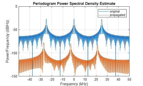
For this wideband signal, you can see that the magnitude of the Doppler shift increases with frequency. In contrast, for narrowband signals, the Doppler shift is assumed constant over the band.