Connecting the Radar Equation to Waveform-Level Simulation

R2026b

Since R2026b

This example demonstrates how to configure the models provided in the Phased Array System Toolbox and Radar Toolbox so that the power levels of the signals produced agree with the predictions of the radar equation.

The unifying thread is signal-to-noise ratio (SNR)—the quantity that ultimately drives most radar performance metrics. A simple scenario is used to compute the SNR three different ways, validating that the models behave as expected:

1. Power-budget calculation via the radar equation

2. I/Q signal-level simulation using individual propagation modeling objects

3. Equivalent signal-level model with the radarTransceiver object

By the end, you will have a clear, side-by-side view of how high-level radar concepts translate into executable MATLAB code and how different modeling fidelity levels yield the same core SNR insight. This example clearly explains the mapping between terms in the radar equation, individual propagation modeling objects, and properties on the radarTransceiver.

For more information on creating waveform level radar models based on power level requirements, see:

• Radar Design Part II: From Radar Data to IQ Signal Synthesis

Monostatic Radar Model

Many variations of a high level block diagram for a monostatic radar can be found. The following schematic shows the model used throughout this example and is typical of monostatic radar models considered in MATLAB.

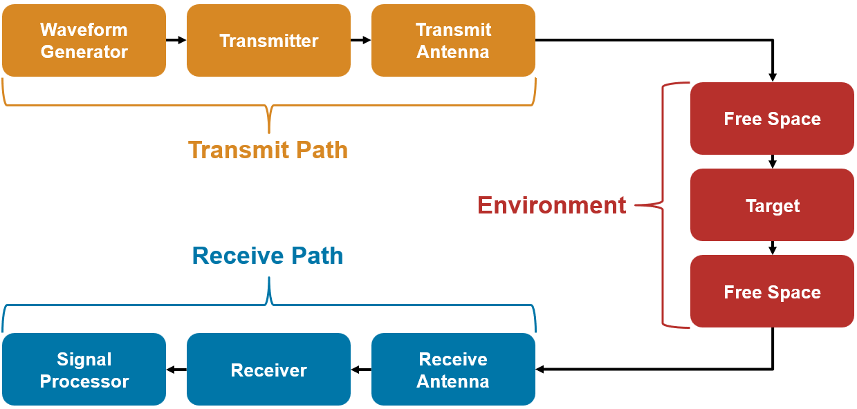
This model does not represent all radar systems and makes many simplifying assumptions - the channel in this case is particularly simple to align with the radar equation which is written for only a single radar target and typically ignores clutter and other environmental effects.

The model presented here is powerful because it maps directly to groups of terms in the radar equation, individual propagation modeling objects, as well as properties on the radarTransceiver. The remainder of this example discusses that mapping and how each of these components impacts the SNR of the final signal received by a radar system.

Signal Model

The waveform-level models used throughout this example employ a complex baseband signal representation. Signal power is proportional to the squared magnitude of the complex waveform, so the waveform magnitude may be interpreted as the square root of power. This convention is used consistently throughout the radar signal chain, including RF circuits, antennas, propagation channels, and receiver processing.

Under this abstraction, the toolbox tracks signal power rather than physical quantities such as voltage, current, or electric field strength. Impedance effects are not modeled explicitly, and perfect matching is assumed throughout the system. As a result, the same waveform magnitude represents the same signal power regardless of whether the signal is interpreted as a guided waveform in a circuit or a radiated electromagnetic wave in space. This power-based representation allows simulated waveform amplitudes to remain consistent with radar-equation and link-budget calculations while simplifying the underlying signal model.

Simple Radar Scenario

The scenario is a target with a radar cross section (RCS) of 1 m² at a range of 5 km along the x-axis. The system is a monostatic radar operating at 5 GHz, 50 MHz bandwidth, with a peak transmit power of 20 kW, pulse width of 100 μs, and pulse repetition frequency (PRF) of 2000. The same cosine antenna element is used for both transmit and receive. The receiver sampling rate is 50 MHz and the noise temperature for the single receive channel is 400 K.

SNR Calculation: Radar Equation

The goal of this section is to estimate the single-pulse matched-filter SNR of the target using the classic radar SNR equation. The derivation is not covered here; for additional information see Radar Equation.

The received SNR given by the classic radar equation is

$$SNR=\frac{P_t\tau G_t{G}_r{\lambda }^2\sigma }{{\left(4\pi \right)}^{3}kT{R}_t^2{R}_r^2}$$

where the terms in the equation are:

• $P_t$ = Peak transmit power in watts.

• $\tau$ = Transmit duration in seconds.

• $G_t$ = Transmit antenna gain.

• $G_r$ = Receive antenna gain.

• $\lambda$ = Signal wavelength.

• $\sigma$ = Target radar cross section (RCS).

• $k$ = Boltzmann constant.

• $T$ = System noise temperature.

• $R_t$ = Distance from transmitter to target.

• $R_r$ = Distance from receiver to target.

Total system loss is sometimes included in this equation but is ignored in this case.

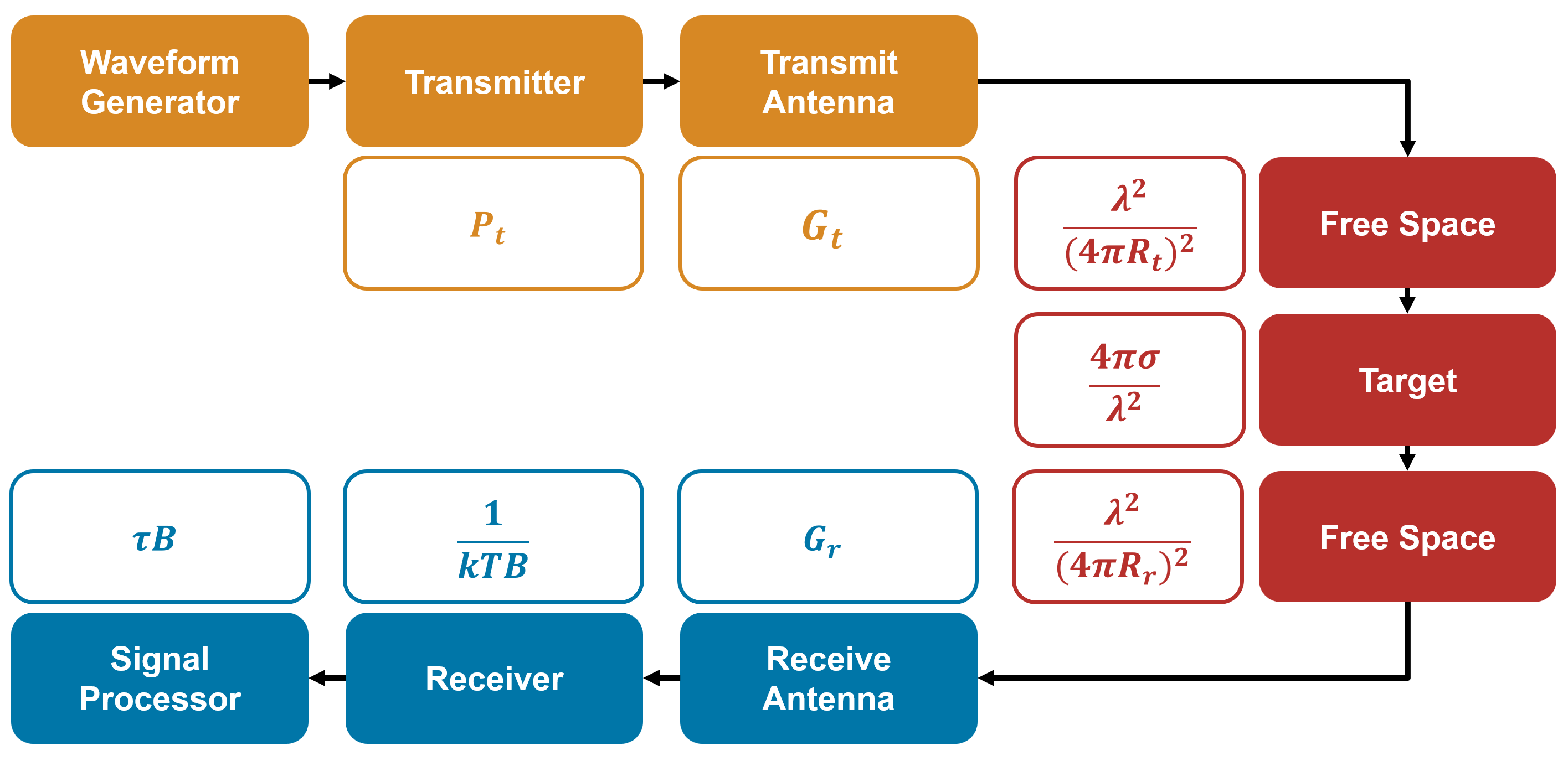
There are numerous ways to rearrange the terms of the radar equation. In this case it is illustrative to rearrange the equation to group terms in order to map them to the monostatic radar schematic shown in the previous section.

$$SNR=P_t*G_t*\frac{{\lambda }^2}{{\left(4\pi R_t\right)}^2}*\frac{4\pi \sigma }{{\lambda }^2}*\frac{{\lambda }^2}{{\left(4\pi R_r\right)}^2}*G_r*\frac{1}{kTB}*\tau B$$

Notice there is one new term $B$ which represents signal bandwidth. The term $\tau B$ gives the matched filter gain - however bandwidth increases both noise power and matched filter gain equally and is therefore excluded from the more compact SNR equation. Each of these terms can be directly mapped to one of the blocks in the monostatic radar model. The figure below shows the monostatic radar model mapped to terms in the formulation of the radar equation presented above.

SNR From Radar Equation

This section calculates the SNR from the radar equation using system-level parameters for the theoretical radar and scenario. The values defined here are taken as ground truth for all else that follows. The goal is to map these values to the three parallel SNR workflows outlined in the introduction.

Radar System and Scenario Parameters

Initialize the random number generator to ensure reproducibility.

rng("default");

Set the key operating parameters.

fc = 5e9;                            % Center frequency (Hz)
lambda = freq2wavelen(fc);           % Wavelength (m)
peakPower = 20e3;                    % Peak transmit power (W)
pulseWidth = 1e-4;                   % Pulse width of radar waveform (s)
antennaGain = 9.0309;                % Antenna gain (dBi)
noiseTemp = 400;                     % Noise temperature for receiver channel
bandWidth = 50e6;                    % Waveform bandwidth (Hz)
fs = bandWidth;                      % Receiver sampling rate (Hz)
pri = 5e-4;                          % Pulse repetition interval (s)
prf = 1/pri;                         % Pulse repetition frequency (Hz)
targetRCS = 1;                       % Target radar cross section (m^2)
targetRange = 5e3;                   % Target range (m)

A few adjustments ensure that the models in subsequent sections are configured properly.

The waveform object requires that the sample rate is an integer multiple of PRF.

fs = round(fs/prf)*prf;

Snap the target range to an integer multiple of the range bin size. This is not a system requirement, but it avoids straddling losses in the matched filter that are not accounted for in the radar equation.

c = physconst("LightSpeed");
binSize = c/fs;
targetRange = round(targetRange/binSize)*(binSize);

Define the radar and target positions for the signal propagation section.

radarPos = [0;0;0];
targetPos = [targetRange;0;0];

SNR Estimate

Call radareqsnr to obtain the single-pulse matched-filter SNR estimate.

snrRadarEquation = radareqsnr(lambda,targetRange,peakPower,pulseWidth, ...
    RCS=targetRCS,Gain=antennaGain,Ts=noiseTemp)

snrRadarEquation = 
18.2707

SNR Calculation: Propagation Modeling Objects

The models from the Phased Array System Toolbox are fundamental building blocks of many RF/radar workflows in MATLAB. They are also leveraged by the expanded capabilities offered by the Radar Toolbox.

The figure below maps each block in the monostatic radar model to the corresponding model that is used to represent it.

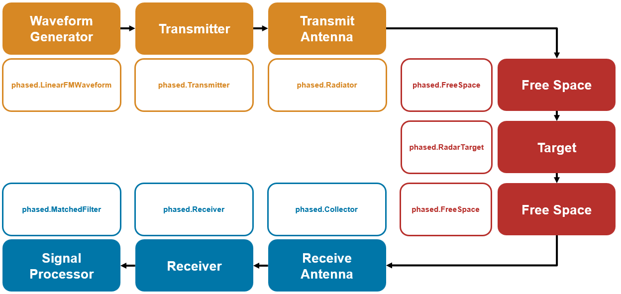
The following sections step clockwise through the block diagram, starting with the Waveform Generator, defining each corresponding object with properties that match the system level parameters from the radar equation section.

At each stage, the signal power out of the corresponding object is compared against the prediction from the radar equation.

At the end of this section, the overall SNR of the propagated signal is measured and verified against the radar equation prediction.

Waveform Generator

The waveform generator is responsible for generating a unit-voltage complex baseband waveform. This is the beginning of any radar RF chain.

The radar equation does not dictate the power level out of the waveform generator directly. The waveform generator produces a unit-power signal (1 W), which the transmitter then amplifies to the peak transmit power.

expectedPower = 1;

In this example the phased.LinearFMWaveform is used as the waveform generator. The specific waveform choice does not affect this power-level analysis.

waveform = phased.LinearFMWaveform(SampleRate=fs, ...
    SweepBandwidth=bandWidth,PulseWidth=pulseWidth, ...
    PRF=prf,SweepInterval="Symmetric");

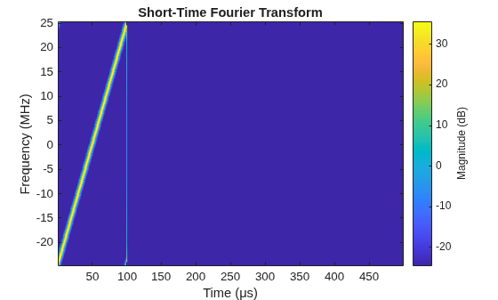
The spectrogram shows the time-frequency dependency of the waveform and can be computed using the stft function.

initSig = waveform();
stft(initSig,fs);

Waveform power over time is shown in the following plot.

t = (0:length(initSig)-1)*1/fs;
helperPlotPowerComparison(t,initSig,expectedPower, ...
    "Waveform Generator Output","Signal Power: Waveform Generator Output");

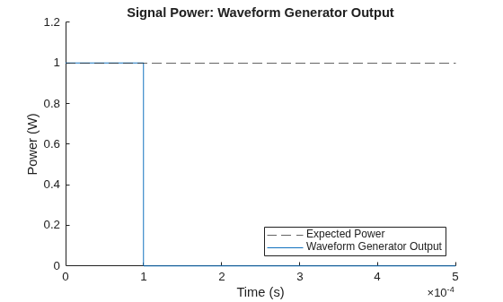
The signal power from the waveform generator matches our expectations while transmission is occurring. This plot is replicated for each step in the propagation chain.

Transmitter

The transmitter amplifies the generated waveform. It is expected that the signal coming out of the transmitter model has a peak power equal to the peak power value specified in the radar equation.

expectedTxPower = peakPower;

The phased.Transmitter models amplification of the input waveform. Its Gain property can apply additional gain not included in the antenna model. Here all antenna gain is modeled in the transmit antenna (next section), so Gain is set to 0.

transmitter = phased.Transmitter(PeakPower=peakPower,Gain=0);

Pass the signal through the transmitter.

txSig = transmitter(initSig);

Verify that the output power matches the expected peak transmit power.

helperPlotPowerComparison(t,txSig,expectedTxPower, ...
    "Transmitter Output","Signal Power: Transmitter Output");

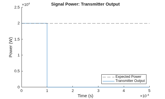
Transmit Antenna

The transmitter output signal is radiated into free space through the transmit antenna. The phased.Radiator models the far-field radiation of a signal from an antenna or antenna array.

The signal output from the transmit antenna model represents equivalent isotropically radiated power (EIRP). This is the power that would need to be radiated by an isotropic element to have the equivalent power density in the transmit direction. For an isotropic element, output power would equal the transmit power.

The antenna gain value in the radar equation section was chosen to match the directivity of this antenna element. The expected output power toward the target equals the transmit power multiplied by the antenna gain.

expectedRadPower = expectedTxPower*db2pow(antennaGain);

The system uses a cosine antenna element.

antenna = phased.CosineAntennaElement(CosinePower=[1.5 1.5]);

Calculate the angle from the radar to the target. The target was placed on the x-axis, which is the direction of maximum gain for this antenna. Power-level analysis typically assumes maximum antenna gain.

[~,targetAng] = rangeangle(targetPos,radarPos);

Verify the total antenna gain. The original specification was set to match this value. In practice, antenna gain requirements drive the antenna design.

disp(antenna.directivity(fc,targetAng));

    9.0309

Plot 3D radiation pattern of the antenna element.

ax = axes(figure);
antenna.pattern(fc,Parent=ax);

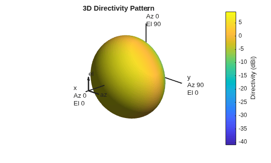
The phased.Radiator applies the far-field radiation pattern to the signal. Setting SensorGainMeasure to "dBi" is critical—it ensures that the gain is referenced to an isotropic radiator so that the output power agrees with the radar equation.

radiator = phased.Radiator(Sensor=antenna, ...
    OperatingFrequency=fc,SensorGainMeasure="dBi");

Propagate the signal out of the radiator toward boresight (direction of maximum gain).

radSig = radiator(txSig,targetAng);

Confirm that the radiated power matches the radar equation prediction.

helperPlotPowerComparison(t,radSig,expectedRadPower, ...
    "Radiator Output","Signal Power: Radiator Output");

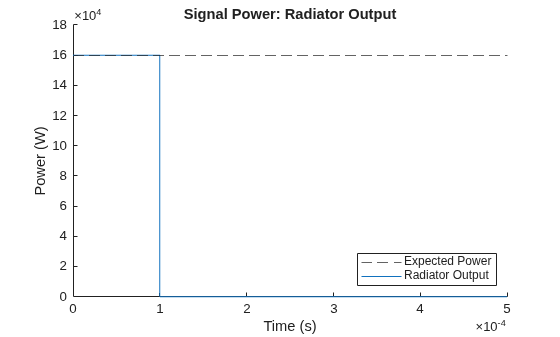
Propagation: Transmitter To Target

Radar signal propagation is fundamentally electromagnetic wave propagation. Several MATLAB features are available for nontrivial RF propagation scenarios, but this example assumes free-space propagation with no attenuation, clutter, or multi-path.

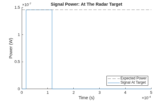
The signal output from the propagation model represents the power that would be intercepted by an isotropic receiver at the target location. The expected power is calculated by multiplying the output power from the radiator by the free space propagation loss.

expectedTargetPropPower = expectedRadPower/db2pow(fspl(targetRange,lambda));

Model free-space propagation with the phased.FreeSpace System object.

fsTxTargChannel = phased.FreeSpace(OperatingFrequency=fc,SampleRate=fs,FractionalDelayMethod='FIR');

Generate the signal arriving at the target assuming that both radar and target are stationary.

targPropSig = fsTxTargChannel(radSig,radarPos,targetPos,[0;0;0],[0;0;0]);

Verify that the signal power at the target matches the free-space path loss prediction.

helperPlotPowerComparison(t,targPropSig,expectedTargetPropPower, ...
    "Signal At Target","Signal Power: At The Radar Target");

Target Reflection

Some of the power arriving at the target is reflected in the direction of the radar receiver.

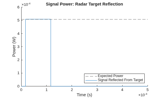
The reflected signal represents the power re-radiated toward the receive antenna. This is analogous to the radiator output: the RCS acts as an effective aperture that captures incident power and re-radiates it. The expected reflected power equals the incident power times the RCS gain term from the radar equation.

expectedTargetReflPower = expectedTargetPropPower*db2pow(aperture2gain(targetRCS,lambda));

The phased.RadarTarget object models this reflection. The RCS is defined as a constant value across all incident and scattering angles.

target = phased.RadarTarget(OperatingFrequency=fc,MeanRCS=targetRCS);

Simulate reflection off of the target.

targReflSig = target(targPropSig);

Confirm that the reflected power agrees with the RCS gain term from the radar equation.

helperPlotPowerComparison(t,targReflSig,expectedTargetReflPower, ...
    "Signal Reflected From Target","Signal Power: Radar Target Reflection");

Propagation: Target To Receiver

The same model is used to propagate the signal from the target to the receiver as was used for propagating the signal from the transmitter to the target.

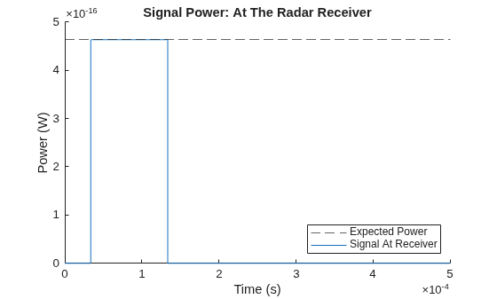
fsTargRxChannel = phased.FreeSpace(OperatingFrequency=fc,SampleRate=fs,FractionalDelayMethod='FIR');

This time propagation is modeled using the target as the origin and the radar as the destination. In this case, the power out of the propagation channel represents the power arriving at an isotropic receiver at the radar location.

expectedRxPropPower = expectedTargetReflPower/db2pow(fspl(targetRange,lambda));
rxPropSig = fsTargRxChannel(targReflSig,targetPos,radarPos,[0;0;0],[0;0;0]);

Verify the signal power arriving at the receiver after return-path propagation loss.

helperPlotPowerComparison(t,rxPropSig,expectedRxPropPower, ...
    "Signal At Receiver","Signal Power: At The Radar Receiver");

Receive Antenna

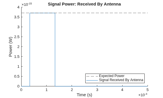
The propagated signal is collected by the receive antenna. The power of the signal arriving at the antenna represents the power that would be intercepted by an isotropic receiver. The phased.Collector applies the antenna gain to determine the received signal power from the target direction.

expectedColPower = expectedRxPropPower*db2pow(antennaGain);

The phased.Collector is the receive-side counterpart of the phased.Radiator. Because this is a monostatic system, the same antenna model is reused. Just like the radiator, the SensorGainMeasure property must again be set to "dBi" so that the results agree with the radar equation.

collector = phased.Collector(Sensor=antenna, ...
    OperatingFrequency=fc,SensorGainMeasure="dBi");

Pass the signal through the collector to simulate reception of the plane wave arriving from the target direction.

collectSig = collector(rxPropSig,targetAng);

The collected signal power is compared to our expectations.

helperPlotPowerComparison(t,collectSig,expectedColPower, ...
    "Signal Received By Antenna","Signal Power: Received By Antenna");

Receiver

The Receiver block is the final stage before signal processing. The phased.Receiver object simulates thermal noise added by the receive chain. It is constructed using the per-channel noise temperature specified above. The noise bandwidth is derived from the sample rate, so the SampleRate property must be specified. Receiver Gain is set to zero to simplify the analysis, but this property can be set to any value without affecting the final SNR because noise and signal are subjected to the same gain value.

receiver = phased.ReceiverPreamp(NoiseMethod="Noise temperature", ...
    ReferenceTemperature=noiseTemp,SampleRate=fs,Gain=0);

Because noise and signal are difficult to separate, first verify that the noise power alone meets expectations by passing a zero signal through the receiver.

emptyIn = zeros(size(collectSig));
noiseOut = receiver(emptyIn);

The expected noise power follows directly from the radar equation noise term.

expectedNoisePower = physconst("Boltzmann")*noiseTemp*bandWidth

expectedNoisePower = 
2.7613e-13

The measured noise power closely matches the prediction, confirming proper receiver noise modeling.

signalNoisePower = rms(noiseOut)^2

signalNoisePower = 
2.7380e-13

With noise power confirmed, pass the actual signal through the receiver to add thermal noise.

rxSig = receiver(collectSig);

Signal Processor

This section applies signal processing and measures the final SNR of the propagated signal.

Apply a matched filter to increase output SNR and improve detectability.

mfCoeff = waveform.getMatchedFilter();
mf = phased.MatchedFilter(Coefficients=mfCoeff);

Pass the signal through the matched filter.

outSig = mf(rxSig);

Remove the transient portion of the filtered signal as well as the latency introduced by the free space propagation model.

nCoeff = length(mfCoeff);
latency = nCoeff + fsTxTargChannel.OutputSignalLatency + fsTargRxChannel.OutputSignalLatency;
outSig = outSig(latency+1:end);

Converting sample time to distance and plotting the matched filter output, the peak due to the radar target is clearly visible at the expected range.

helperPlotMatchedFilterResults(outSig,t,latency,targetRange);

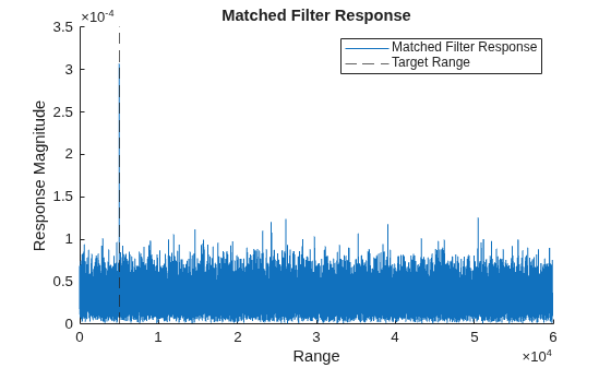
The power of the peak is used to represent the final signal power, and the remaining samples provide a noise estimate. The resulting SNR is compared to the radar equation prediction.

[signal,sigidx] = max(outSig);
noise = outSig(sigidx+100:end);
snrPhasedObjects = pow2db(abs(signal)^2/rms(noise)^2)

snrPhasedObjects = 
18.3596

This matches very closely with the value predicted by the radar equation.

SNR Calculation: radarTransceiver

The radarTransceiver models an entire monostatic radar system and can be used with radarScenario. It is composed of the same building blocks defined in the previous section.

Similarly to the mapping done for the radar equation and individual blocks, the figure below maps the monostatic radar model schematic to properties on the radarTransceiver.

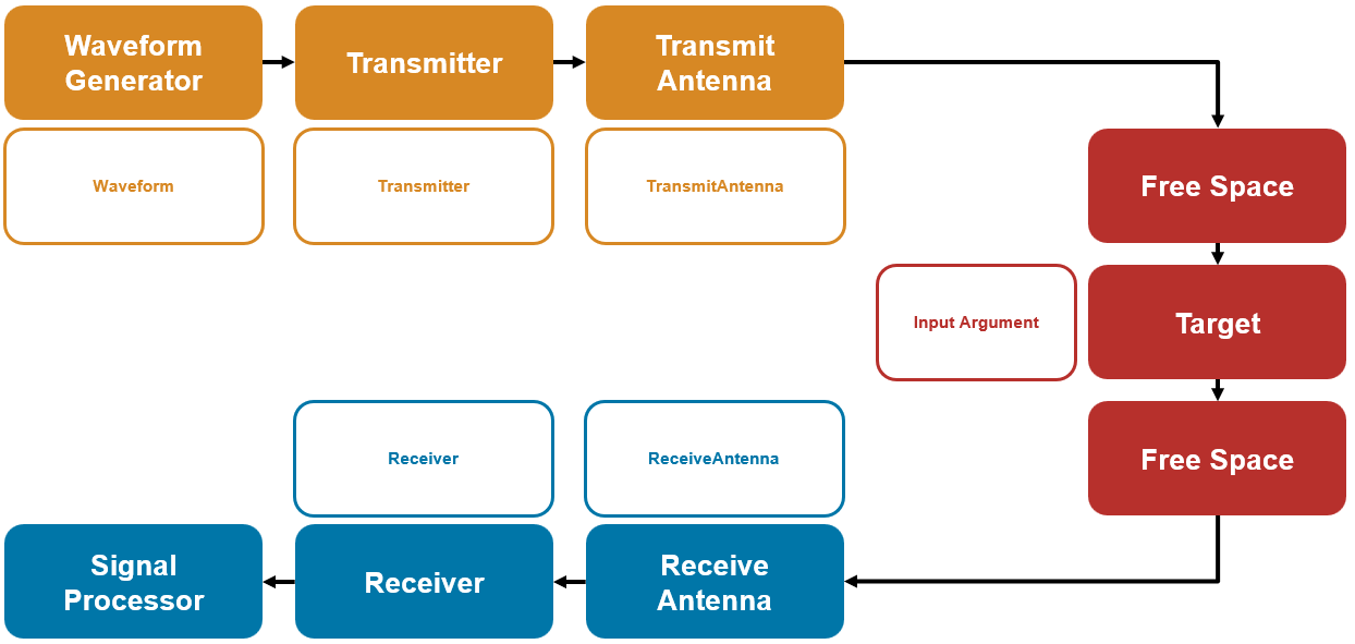
Notice that the free space propagation, radar target, and signal processor blocks do not map directly to properties on the radarTransceiver. The free space propagation is used internally and cannot be specified. The radar target is input to the radar transceiver object and is not a property of the object itself. The signal processor is not a property because the output of the radar transceiver is raw IQ data - signal processing is applied after the radar transceiver outputs this data.

Call radarTransceiver Object

Because the individual objects were already defined in the previous section, constructing the radarTransceiver is straightforward - the underlying models are exactly the same.

rdr = radarTransceiver(Waveform=waveform,Transmitter=transmitter, ...
    TransmitAntenna=radiator,ReceiveAntenna=collector,Receiver=receiver)

rdr = 
  radarTransceiver with properties:

                Waveform: [1×1 phased.LinearFMWaveform]
             Transmitter: [1×1 phased.Transmitter]
         TransmitAntenna: [1×1 phased.Radiator]
          ReceiveAntenna: [1×1 phased.Collector]
                Receiver: [1×1 phased.ReceiverPreamp]
      MechanicalScanMode: 'None'
      ElectronicScanMode: 'None'
        MountingLocation: [0 0 0]
          MountingAngles: [0 0 0]
    NumRepetitionsSource: 'Property'
          NumRepetitions: 1
       RangeLimitsSource: 'Property'
             RangeLimits: [0 Inf]
         RangeOutputPort: false
          TimeOutputPort: false

The target is not specified as a property on the radar model - instead it is an input to the function that generates the signal data. Define the target information as a struct - this is the format expected as an input to the radarTransceiver.

rcsSig = rcsSignature(Azimuth=[-180 180], ...
    Elevation=[-90 90],Pattern=pow2db(target.MeanRCS)*ones(2,2));
targetStruct = struct('Position',targetPos,'Velocity',[0;0;0],'Signatures',rcsSig);

Invoke the radarTransceiver by passing targetStruct and the reception time. The time is relative to the start of the simulation—here the time is set to one pulse repetition interval (PRI).

timeRx = 1/waveform.PRF;
rtSig = rdr(targetStruct,timeRx);

Signal processing is performed identically to the previous section. After generating the received waveform, pass the signal through the matched filter.

rtOutSig = mf(rtSig);

Remove the transient portion of the filtered signal.

rtOutSig = rtOutSig(nCoeff+1:end);

Converting sample time to distance and plotting the matched filter output, the peak due to the radar target is clearly visible at the expected range.

helperPlotMatchedFilterResults(rtOutSig,t,nCoeff,targetRange);

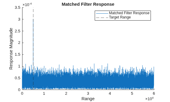
Finally, perform the same analysis for the estimate of the SNR.

[signal,sigidx] = max(rtOutSig);
noise = rtOutSig(sigidx+100:end);
snrRadarTransceiver = pow2db(abs(signal)^2/rms(noise)^2)

snrRadarTransceiver = 
18.1771

The SNR of the output from the radarTransceiver closely matches the prediction of the radar equation and the equivalent signal propagation chain using the individual models.

Conclusion

This example looked at three modeling approaches—the radar equation, individual propagation modeling objects, and the radarTransceiver—and demonstrated how each of these modeling approaches is connected. SNR was used as the common thread to confirm agreement between each approach.

The final figure below shows each of the SNR values side by side.

helperPlotFinalResults(snrRadarEquation,snrPhasedObjects,snrRadarTransceiver);

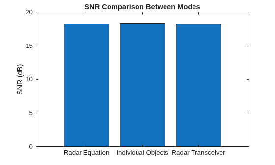
The SNR values from all three approaches agree within ~0.5 dB, validating the transition from classic radar equation parameters to waveform-level simulation with the radarTransceiver sensor model.

Helper Functions

function helperPlotPowerComparison(t,signalMagnitude,expectedPower,signalName,titleStr)
    % Plot a comparison between the propagated and expected signal power.
    signalPower = abs(signalMagnitude.^2);
    ax = axes(figure);
    hold(ax,"on");
    yline(expectedPower,DisplayName="Expected Power",LineStyle="--");
    plot(ax,t,signalPower,DisplayName=signalName);
    ylabel(ax,"Power (W)");
    xlabel(ax,"Time (s)");
    title(ax,titleStr);
    legend(ax,Location="southeast");
end

function helperPlotFinalResults(snrRadarEquation,snrPhasedObjects,snrRadarTransceiver)
    % Plot SNR comparison between the three models.
    ax = axes(figure);
    bar(ax,["Radar Equation","Individual Objects","Radar Transceiver"], ...
        [snrRadarEquation,snrPhasedObjects,snrRadarTransceiver]);
    title(ax,"SNR Comparison Between Modes");
    ylabel(ax,"SNR (dB)");
end

function helperPlotMatchedFilterResults(outSig,t,latency,targetRange)
    % Plot the results of the matched filter output.
    range = t(1:end-latency)*physconst("LightSpeed")/2;
    ax = axes(figure);
    hold(ax,"on");
    plot(ax,range,abs(outSig),DisplayName="Matched Filter Response");
    xline(ax,targetRange,DisplayName="Target Range",LineStyle="--");
    ylabel(ax,"Response Magnitude");
    xlabel(ax,"Range");
    title(ax,'Matched Filter Response');
    legend(ax);
end