validatemodel
Validate quality of compact credit scorecard model
Syntax
Description
Stats = validatemodel(csc,data)compactCreditScorecard model for the data set specified using
the argument data.
[
specifies options using one or more name-value pair arguments in addition to
the input arguments in the previous syntax and returns the outputs
Stats,T]
= validatemodel(___,Name,Value)Stats and T.
[
specifies options using one or more name-value pair arguments in addition to
the input arguments in the previous syntax and returns the outputs
Stats,T,hf]
= validatemodel(___,Name,Value)Stats and T and the figure
handle hf to the CAP, ROC, and KS plots.
Examples
Compute model validation statistics for a compact credit scorecard model.
To create a compactCreditScorecard object, you must first develop a credit scorecard model using a creditscorecard object.
Create a creditscorecard object using the CreditCardData.mat file to load the data (using a dataset from Refaat 2011).
load CreditCardData.mat
sc = creditscorecard(data, 'IDVar','CustID')
sc =
  creditscorecard with properties:

                GoodLabel: 0
              ResponseVar: 'status'
               WeightsVar: ''
                 VarNames: {'CustID'  'CustAge'  'TmAtAddress'  'ResStatus'  'EmpStatus'  'CustIncome'  'TmWBank'  'OtherCC'  'AMBalance'  'UtilRate'  'status'}
        NumericPredictors: {'CustAge'  'TmAtAddress'  'CustIncome'  'TmWBank'  'AMBalance'  'UtilRate'}
    CategoricalPredictors: {'ResStatus'  'EmpStatus'  'OtherCC'}
           BinMissingData: 0
                    IDVar: 'CustID'
            PredictorVars: {'CustAge'  'TmAtAddress'  'ResStatus'  'EmpStatus'  'CustIncome'  'TmWBank'  'OtherCC'  'AMBalance'  'UtilRate'}
                     Data: [1200×11 table]
Perform automatic binning using the default options. By default, autobinning uses the Monotone algorithm.
sc = autobinning(sc);
Fit the model.
sc = fitmodel(sc);
1. Adding CustIncome, Deviance = 1490.8527, Chi2Stat = 32.588614, PValue = 1.1387992e-08
2. Adding TmWBank, Deviance = 1467.1415, Chi2Stat = 23.711203, PValue = 1.1192909e-06
3. Adding AMBalance, Deviance = 1455.5715, Chi2Stat = 11.569967, PValue = 0.00067025601
4. Adding EmpStatus, Deviance = 1447.3451, Chi2Stat = 8.2264038, PValue = 0.0041285257
5. Adding CustAge, Deviance = 1441.994, Chi2Stat = 5.3511754, PValue = 0.020708306
6. Adding ResStatus, Deviance = 1437.8756, Chi2Stat = 4.118404, PValue = 0.042419078
7. Adding OtherCC, Deviance = 1433.707, Chi2Stat = 4.1686018, PValue = 0.041179769

Generalized linear regression model:
    logit(status) ~ 1 + CustAge + ResStatus + EmpStatus + CustIncome + TmWBank + OtherCC + AMBalance
    Distribution = Binomial

Estimated Coefficients:
                   Estimate       SE       tStat       pValue
                   ________    ________    ______    __________

    (Intercept)    0.70239     0.064001    10.975    5.0538e-28
    CustAge        0.60833      0.24932      2.44      0.014687
    ResStatus        1.377      0.65272    2.1097      0.034888
    EmpStatus      0.88565        0.293    3.0227     0.0025055
    CustIncome     0.70164      0.21844    3.2121     0.0013179
    TmWBank         1.1074      0.23271    4.7589    1.9464e-06
    OtherCC         1.0883      0.52912    2.0569      0.039696
    AMBalance        1.045      0.32214    3.2439     0.0011792


1200 observations, 1192 error degrees of freedom
Dispersion: 1
Chi^2-statistic vs. constant model: 89.7, p-value = 1.4e-16
Format the unscaled points.
sc = formatpoints(sc, 'PointsOddsAndPDO',[500,2,50]);Convert the creditscorecard object into a compactCreditScorecard object. A compactCreditScorecard object is a lightweight version of a creditscorecard object that is used for deployment purposes.
csc = compactCreditScorecard(sc);
Validate the compact credit scorecard model by generating the CAP, ROC, and KS plots. This example uses the training data. However, you can use any validation data, as long as:
The data has the same predictor names and predictor types as the data used to create the initial
creditscorecardobject.The data has a response column with the same name as the
'ResponseVar'property in the initialcreditscorecardobject.The data has a weights column (if weights were used to train the model) with the same name as
'WeightsVar'property in the initialcreditscorecardobject.
[Stats,T] = validatemodel(csc,data,'Plot',{'CAP','ROC','KS'});

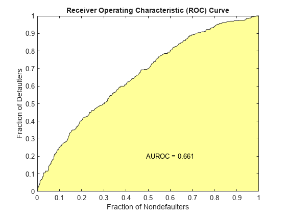
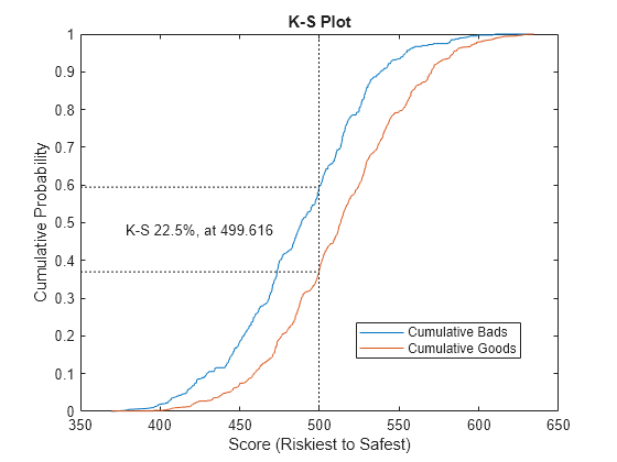
disp(Stats)
            Measure              Value
    ________________________    _______

    {'Accuracy Ratio'      }    0.32258
    {'Area under ROC curve'}    0.66129
    {'KS statistic'        }     0.2246
    {'KS score'            }     499.62
disp(T(1:15,:))
    Scores    ProbDefault    TrueBads    FalseBads    TrueGoods    FalseGoods    Sensitivity    FalseAlarm      PctObs
    ______    ___________    ________    _________    _________    __________    ___________    __________    __________

    369.54      0.75313          0           1           802          397                 0     0.0012453     0.00083333
    378.19      0.73016          1           1           802          396         0.0025189     0.0012453      0.0016667
    380.28      0.72444          2           1           802          395         0.0050378     0.0012453         0.0025
    391.49      0.69234          3           1           802          394         0.0075567     0.0012453      0.0033333
    395.57      0.68017          4           1           802          393          0.010076     0.0012453      0.0041667
    396.14      0.67846          4           2           801          393          0.010076     0.0024907          0.005
    396.45      0.67752          5           2           801          392          0.012594     0.0024907      0.0058333
    398.61      0.67094          6           2           801          391          0.015113     0.0024907      0.0066667
    398.68      0.67072          7           2           801          390          0.017632     0.0024907         0.0075
    401.33      0.66255          8           2           801          389          0.020151     0.0024907      0.0083333
    402.66      0.65842          8           3           800          389          0.020151      0.003736      0.0091667
    404.25      0.65346          9           3           800          388           0.02267      0.003736           0.01
    404.73      0.65193          9           4           799          388           0.02267     0.0049813       0.010833
    405.53      0.64941         11           4           799          386          0.027708     0.0049813         0.0125
     405.7      0.64887         11           5           798          386          0.027708     0.0062267       0.013333
Compute model validation statistics for a compact credit scorecard model with weights.
To create a compactCreditScorecard object, you must first develop a credit scorecard model using a creditscorecard object.
Use the CreditCardData.mat file to load the data (dataWeights) that contains a column (RowWeights) for the weights (using a dataset from Refaat 2011).
load CreditCardData.matCreate a creditscorecard object using the optional name-value argument WeightsVar.
sc = creditscorecard(dataWeights,'IDVar','CustID',WeightsVar="RowWeights")
sc =
  creditscorecard with properties:

                GoodLabel: 0
              ResponseVar: 'status'
               WeightsVar: 'RowWeights'
                 VarNames: {'CustID'  'CustAge'  'TmAtAddress'  'ResStatus'  'EmpStatus'  'CustIncome'  'TmWBank'  'OtherCC'  'AMBalance'  'UtilRate'  'RowWeights'  'status'}
        NumericPredictors: {'CustAge'  'TmAtAddress'  'CustIncome'  'TmWBank'  'AMBalance'  'UtilRate'}
    CategoricalPredictors: {'ResStatus'  'EmpStatus'  'OtherCC'}
           BinMissingData: 0
                    IDVar: 'CustID'
            PredictorVars: {'CustAge'  'TmAtAddress'  'ResStatus'  'EmpStatus'  'CustIncome'  'TmWBank'  'OtherCC'  'AMBalance'  'UtilRate'}
                     Data: [1200×12 table]
Perform automatic binning. By default, autobinning uses the Monotone algorithm.
sc = autobinning(sc)
sc =
  creditscorecard with properties:

                GoodLabel: 0
              ResponseVar: 'status'
               WeightsVar: 'RowWeights'
                 VarNames: {'CustID'  'CustAge'  'TmAtAddress'  'ResStatus'  'EmpStatus'  'CustIncome'  'TmWBank'  'OtherCC'  'AMBalance'  'UtilRate'  'RowWeights'  'status'}
        NumericPredictors: {'CustAge'  'TmAtAddress'  'CustIncome'  'TmWBank'  'AMBalance'  'UtilRate'}
    CategoricalPredictors: {'ResStatus'  'EmpStatus'  'OtherCC'}
           BinMissingData: 0
                    IDVar: 'CustID'
            PredictorVars: {'CustAge'  'TmAtAddress'  'ResStatus'  'EmpStatus'  'CustIncome'  'TmWBank'  'OtherCC'  'AMBalance'  'UtilRate'}
                     Data: [1200×12 table]
Fit the model.
sc = fitmodel(sc);
1. Adding CustIncome, Deviance = 764.3187, Chi2Stat = 15.81927, PValue = 6.968927e-05
2. Adding TmWBank, Deviance = 751.0215, Chi2Stat = 13.29726, PValue = 0.0002657942
3. Adding AMBalance, Deviance = 743.7581, Chi2Stat = 7.263384, PValue = 0.007037455

Generalized linear regression model:
    logit(status) ~ 1 + CustIncome + TmWBank + AMBalance
    Distribution = Binomial

Estimated Coefficients:
                   Estimate       SE       tStat       pValue
                   ________    ________    ______    __________

    (Intercept)    0.70642     0.088702     7.964    1.6653e-15
    CustIncome      1.0268      0.25758    3.9862    6.7132e-05
    TmWBank         1.0973      0.31294    3.5063     0.0004543
    AMBalance       1.0039      0.37576    2.6717     0.0075464


1200 observations, 1196 error degrees of freedom
Dispersion: 1
Chi^2-statistic vs. constant model: 36.4, p-value = 6.22e-08
Format the unscaled points.
sc = formatpoints(sc,'PointsOddsAndPDO',[500,2,50]);Convert the creditscorecard object into a compactCreditScorecard object. A compactCreditScorecard object is a lightweight version of a creditscorecard object that is used for deployment purposes.
csc = compactCreditScorecard(sc);
Validate the compact credit scorecard model by generating the CAP, ROC, and KS plots. When you use the optional name-value argument WeightsVar to specify observation (sample) weights in the original creditscorecard object, the T table for validatemodel uses statistics, sums, and cumulative sums that are weighted counts.
This example uses the training data (dataWeights). However, you can use any validation data, as long as:
The data has the same predictor names and predictor types as the data used to create the initial
creditscorecardobject.The data has a response column with the same name as the
'ResponseVar'property in the initialcreditscorecardobject.The data has a weights column (if weights were used to train the model) with the same name as the
WeightsVarproperty in the initialcreditscorecardobject.
[Stats,T] = validatemodel(csc,dataWeights,'Plot',{'CAP','ROC','KS'});
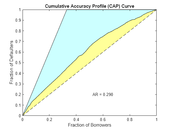
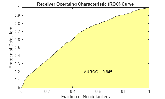
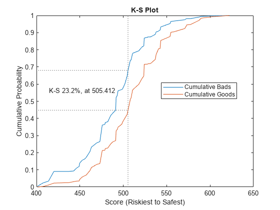
Stats
Stats=4×2 table
            Measure              Value
    ________________________    _______

    {'Accuracy Ratio'      }    0.28972
    {'Area under ROC curve'}    0.64486
    {'KS statistic'        }    0.23215
    {'KS score'            }     505.41
T(1:10,:)
ans=10×9 table
    Scores    ProbDefault    TrueBads    FalseBads    TrueGoods    FalseGoods    Sensitivity    FalseAlarm     PctObs
    ______    ___________    ________    _________    _________    __________    ___________    __________    _________

    401.34      0.66253       1.0788           0       411.95        201.95       0.0053135             0     0.0017542
    407.59      0.64289       4.8363      1.2768       410.67        198.19        0.023821     0.0030995     0.0099405
    413.79      0.62292       6.9469      4.6942       407.25        196.08        0.034216      0.011395      0.018929
    420.04      0.60236       18.459      9.3899       402.56        184.57        0.090918      0.022794      0.045285
    437.27        0.544       18.459      10.514       401.43        184.57        0.090918      0.025523      0.047113
    442.83      0.52481       18.973      12.794       399.15        184.06        0.093448      0.031057      0.051655
    446.19      0.51319       22.396       14.15        397.8        180.64         0.11031      0.034349      0.059426
    449.08      0.50317       24.325      14.405       397.54        178.71         0.11981      0.034968      0.062978
    449.73      0.50095       28.246      18.049        393.9        174.78         0.13912      0.043813      0.075279
    452.44      0.49153       31.511      23.565       388.38        171.52          0.1552      0.057204      0.089557
Compute model validation statistics and assign points for missing data when using the 'BinMissingData' option.
Predictors in a
creditscorecardobject that have missing data in the training set have an explicit bin for<missing>with corresponding points in the final scorecard. These points are computed from the Weight-of-Evidence (WOE) value for the<missing>bin and the logistic model coefficients. For scoring purposes, these points are assigned to missing values and to out-of-range values, and after you convert thecreditscorecardobject to acompactCreditScorecardobject, you can use the final score to compute model validation statistics withvalidatemodel.Predictors in a
creditscorecardobject with no missing data in the training set have no<missing>bin, so no WOE can be estimated from the training data. By default, the points for missing and out-of-range values are set toNaNresulting in a score ofNaNwhen runningscore. For predictors in acreditscorecardobject that have no explicit<missing>bin, use the name-value argument'Missing'informatpointsto specify how the function treats missing data for scoring purposes. After converting thecreditscorecardobject to acompactCreditScorecardobject, you can use the final score to compute model validation statistics withvalidatemodel.
To create a compactCreditScorecard object, you must first develop a credit scorecard model using a creditscorecard object.
Create a creditscorecard object using the CreditCardData.mat file to load dataMissing, a table that contains missing values.
load CreditCardData.mat
head(dataMissing,5)
CustID CustAge TmAtAddress ResStatus EmpStatus CustIncome TmWBank OtherCC AMBalance UtilRate status
______ _______ ___________ ___________ _________ __________ _______ _______ _________ ________ ______
1 53 62 <undefined> Unknown 50000 55 Yes 1055.9 0.22 0
2 61 22 Home Owner Employed 52000 25 Yes 1161.6 0.24 0
3 47 30 Tenant Employed 37000 61 No 877.23 0.29 0
4 NaN 75 Home Owner Employed 53000 20 Yes 157.37 0.08 0
5 68 56 Home Owner Employed 53000 14 Yes 561.84 0.11 0
Use creditscorecard with the name-value argument 'BinMissingData' set to true to bin the missing numeric or categorical data in a separate bin. Apply automatic binning.
sc = creditscorecard(dataMissing,'IDVar','CustID','BinMissingData',true);
sc = autobinning(sc);

disp(sc)
  creditscorecard with properties:

                GoodLabel: 0
              ResponseVar: 'status'
               WeightsVar: ''
                 VarNames: {'CustID'  'CustAge'  'TmAtAddress'  'ResStatus'  'EmpStatus'  'CustIncome'  'TmWBank'  'OtherCC'  'AMBalance'  'UtilRate'  'status'}
        NumericPredictors: {'CustAge'  'TmAtAddress'  'CustIncome'  'TmWBank'  'AMBalance'  'UtilRate'}
    CategoricalPredictors: {'ResStatus'  'EmpStatus'  'OtherCC'}
           BinMissingData: 1
                    IDVar: 'CustID'
            PredictorVars: {'CustAge'  'TmAtAddress'  'ResStatus'  'EmpStatus'  'CustIncome'  'TmWBank'  'OtherCC'  'AMBalance'  'UtilRate'}
                     Data: [1200×11 table]
To make any negative age or income information invalid or "out of range," set a minimum value of zero for 'CustAge' and 'CustIncome'. For scoring and probability-of-default computations, out-of-range values are given the same points as missing values.
sc = modifybins(sc,'CustAge','MinValue',0);
sc = modifybins(sc,'CustIncome','MinValue',0);
Display bin information for numeric data for 'CustAge' that includes missing data in a separate bin labeled <missing>.
bi = bininfo(sc,'CustAge');
disp(bi)
Bin Good Bad Odds WOE InfoValue
_____________ ____ ___ ______ ________ __________
{'[0,33)' } 69 52 1.3269 -0.42156 0.018993
{'[33,37)' } 63 45 1.4 -0.36795 0.012839
{'[37,40)' } 72 47 1.5319 -0.2779 0.0079824
{'[40,46)' } 172 89 1.9326 -0.04556 0.0004549
{'[46,48)' } 59 25 2.36 0.15424 0.0016199
{'[48,51)' } 99 41 2.4146 0.17713 0.0035449
{'[51,58)' } 157 62 2.5323 0.22469 0.0088407
{'[58,Inf]' } 93 25 3.72 0.60931 0.032198
{'<missing>'} 19 11 1.7273 -0.15787 0.00063885
{'Totals' } 803 397 2.0227 NaN 0.087112
Display bin information for categorical data for 'ResStatus' that includes missing data in a separate bin labeled <missing>.
bi = bininfo(sc,'ResStatus');
disp(bi)
Bin Good Bad Odds WOE InfoValue
______________ ____ ___ ______ _________ __________
{'Tenant' } 296 161 1.8385 -0.095463 0.0035249
{'Home Owner'} 352 171 2.0585 0.017549 0.00013382
{'Other' } 128 52 2.4615 0.19637 0.0055808
{'<missing>' } 27 13 2.0769 0.026469 2.3248e-05
{'Totals' } 803 397 2.0227 NaN 0.0092627
For the 'CustAge' and 'ResStatus' predictors, the training data contains missing data (NaNs and <undefined> values. For missing data in these predictors, the binning process estimates WOE values of -0.15787 and 0.026469, respectively.
Because the training data contains no missing values for the 'EmpStatus' and 'CustIncome' predictors, neither predictor has an explicit bin for missing values.
bi = bininfo(sc,'EmpStatus');
disp(bi)
Bin Good Bad Odds WOE InfoValue
____________ ____ ___ ______ ________ _________
{'Unknown' } 396 239 1.6569 -0.19947 0.021715
{'Employed'} 407 158 2.5759 0.2418 0.026323
{'Totals' } 803 397 2.0227 NaN 0.048038
bi = bininfo(sc,'CustIncome');
disp(bi)
Bin Good Bad Odds WOE InfoValue
_________________ ____ ___ _______ _________ __________
{'[0,29000)' } 53 58 0.91379 -0.79457 0.06364
{'[29000,33000)'} 74 49 1.5102 -0.29217 0.0091366
{'[33000,35000)'} 68 36 1.8889 -0.06843 0.00041042
{'[35000,40000)'} 193 98 1.9694 -0.026696 0.00017359
{'[40000,42000)'} 68 34 2 -0.011271 1.0819e-05
{'[42000,47000)'} 164 66 2.4848 0.20579 0.0078175
{'[47000,Inf]' } 183 56 3.2679 0.47972 0.041657
{'Totals' } 803 397 2.0227 NaN 0.12285
Use fitmodel to fit a logistic regression model using Weight of Evidence (WOE) data. fitmodel internally transforms all the predictor variables into WOE values by using the bins found in the automatic binning process. fitmodel then fits a logistic regression model using a stepwise method (by default). For predictors that have missing data, there is an explicit <missing> bin, with a corresponding WOE value computed from the data. When you use fitmodel, the function applies the corresponding WOE value for the <missing> bin when performing the WOE transformation.
[sc,mdl] = fitmodel(sc);
1. Adding CustIncome, Deviance = 1490.8527, Chi2Stat = 32.588614, PValue = 1.1387992e-08
2. Adding TmWBank, Deviance = 1467.1415, Chi2Stat = 23.711203, PValue = 1.1192909e-06
3. Adding AMBalance, Deviance = 1455.5715, Chi2Stat = 11.569967, PValue = 0.00067025601
4. Adding EmpStatus, Deviance = 1447.3451, Chi2Stat = 8.2264038, PValue = 0.0041285257
5. Adding CustAge, Deviance = 1442.8477, Chi2Stat = 4.4974731, PValue = 0.033944979
6. Adding ResStatus, Deviance = 1438.9783, Chi2Stat = 3.86941, PValue = 0.049173805
7. Adding OtherCC, Deviance = 1434.9751, Chi2Stat = 4.0031966, PValue = 0.045414057

Generalized linear regression model:
    logit(status) ~ 1 + CustAge + ResStatus + EmpStatus + CustIncome + TmWBank + OtherCC + AMBalance
    Distribution = Binomial

Estimated Coefficients:
                   Estimate       SE       tStat       pValue
                   ________    ________    ______    __________

    (Intercept)    0.70229     0.063959     10.98    4.7498e-28
    CustAge        0.57421      0.25708    2.2335      0.025513
    ResStatus       1.3629      0.66952    2.0356       0.04179
    EmpStatus      0.88373       0.2929    3.0172      0.002551
    CustIncome     0.73535       0.2159     3.406    0.00065929
    TmWBank         1.1065      0.23267    4.7556    1.9783e-06
    OtherCC         1.0648      0.52826    2.0156      0.043841
    AMBalance       1.0446      0.32197    3.2443     0.0011775


1200 observations, 1192 error degrees of freedom
Dispersion: 1
Chi^2-statistic vs. constant model: 88.5, p-value = 2.55e-16
Scale the scorecard points by the "points, odds, and points to double the odds (PDO)" method using the 'PointsOddsAndPDO' argument of formatpoints. Suppose that you want a score of 500 points to have odds of 2 (twice as likely to be good than to be bad) and that the odds double every 50 points (so that 550 points would have odds of 4).
Display the scorecard showing the scaled points for predictors retained in the fitting model.
sc = formatpoints(sc,'PointsOddsAndPDO',[500 2 50]);
PointsInfo = displaypoints(sc)PointsInfo=38×3 table
Predictors Bin Points
_____________ ______________ ______
{'CustAge' } {'[0,33)' } 54.062
{'CustAge' } {'[33,37)' } 56.282
{'CustAge' } {'[37,40)' } 60.012
{'CustAge' } {'[40,46)' } 69.636
{'CustAge' } {'[46,48)' } 77.912
{'CustAge' } {'[48,51)' } 78.86
{'CustAge' } {'[51,58)' } 80.83
{'CustAge' } {'[58,Inf]' } 96.76
{'CustAge' } {'<missing>' } 64.984
{'ResStatus'} {'Tenant' } 62.138
{'ResStatus'} {'Home Owner'} 73.248
{'ResStatus'} {'Other' } 90.828
{'ResStatus'} {'<missing>' } 74.125
{'EmpStatus'} {'Unknown' } 58.807
{'EmpStatus'} {'Employed' } 86.937
{'EmpStatus'} {'<missing>' } NaN
⋮
Notice that points for the <missing> bin for 'CustAge' and 'ResStatus' are explicitly shown (as 64.9836 and 74.1250, respectively). The function computes these points from the WOE value for the <missing> bin and the logistic model coefficients.
For predictors that have no missing data in the training set, there is no explicit <missing> bin during the training of the model. By default, displaypoints reports the points as NaN for missing data resulting in a score of NaN when you use score. For these predictors, use the name-value pair argument 'Missing' in formatpoints to indicate how missing data should be treated for scoring purposes.
Use compactCreditScorecard to convert the creditscorecard object into a compactCreditScorecard object. A compactCreditScorecard object is a lightweight version of a creditscorecard object that is used for deployment purposes.
csc = compactCreditScorecard(sc);
For the purpose of illustration, take a few rows from the original data as test data and introduce some missing data. Also introduce some invalid, or out-of-range, values. For numeric data, values below the minimum (or above the maximum) are considered invalid, such as a negative value for age (recall that in a previous step, you set 'MinValue' to 0 for 'CustAge' and 'CustIncome'). For categorical data, invalid values are categories not explicitly included in the scorecard, for example, a residential status not previously mapped to scorecard categories, such as "House", or a meaningless string such as "abc123."
This example uses a very small validation data set only to illustrate the scoring of rows with missing and out-of-range values and the relationship between scoring and model validation.
tdata = dataMissing(11:200,mdl.PredictorNames); % Keep only the predictors retained in the model
tdata.status = dataMissing.status(11:200); % Copy the response variable value, needed for validation purposes
% Set some missing values
tdata.CustAge(1) = NaN;
tdata.ResStatus(2) = missing;
tdata.EmpStatus(3) = missing;
tdata.CustIncome(4) = NaN;
% Set some invalid values
tdata.CustAge(5) = -100;
tdata.ResStatus(6) = 'House';
tdata.EmpStatus(7) = 'Freelancer';
tdata.CustIncome(8) = -1;
disp(tdata(1:10,:))
    CustAge     ResStatus      EmpStatus     CustIncome    TmWBank    OtherCC    AMBalance    status
    _______    ___________    ___________    __________    _______    _______    _________    ______

      NaN      Tenant         Unknown          34000         44         Yes        119.8        1
       48      <undefined>    Unknown          44000         14         Yes       403.62        0
       65      Home Owner     <undefined>      48000          6         No        111.88        0
       44      Other          Unknown            NaN         35         No        436.41        0
     -100      Other          Employed         46000         16         Yes       162.21        0
       33      House          Employed         36000         36         Yes       845.02        0
       39      Tenant         Freelancer       34000         40         Yes       756.26        1
       24      Home Owner     Employed            -1         19         Yes       449.61        0
      NaN      Home Owner     Employed         51000         11         Yes       519.46        1
       52      Other          Unknown          42000         12         Yes       1269.2        0
Use validatemodel for a compactCreditScorecard object with the validation data set (tdata).
[ValStats,ValTable] = validatemodel(csc,tdata,'Plot',{'CAP','ROC','KS'});
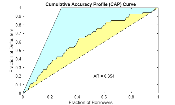
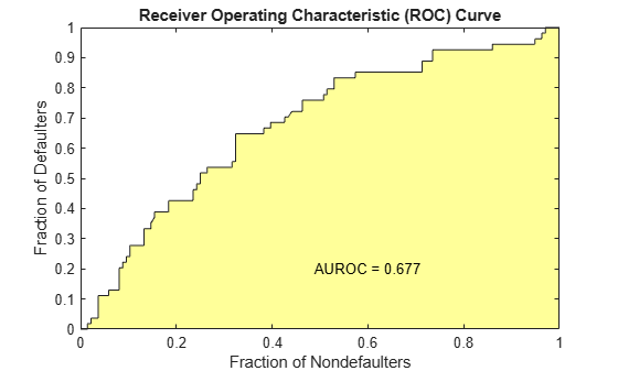
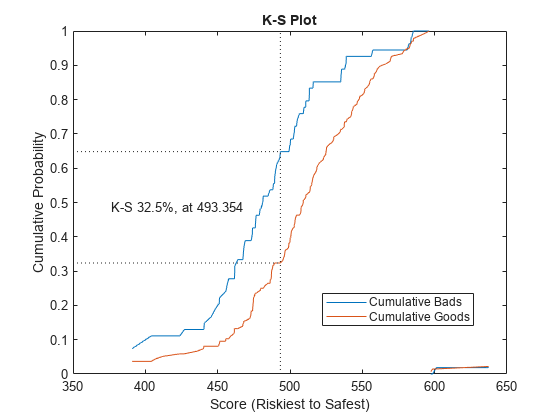
disp(ValStats)
            Measure              Value
    ________________________    _______

    {'Accuracy Ratio'      }    0.35376
    {'Area under ROC curve'}    0.67688
    {'KS statistic'        }    0.32462
    {'KS score'            }     493.35
disp(ValTable(1:10,:))
    Scores    ProbDefault    TrueBads    FalseBads    TrueGoods    FalseGoods    Sensitivity    FalseAlarm     PctObs
    ______    ___________    ________    _________    _________    __________    ___________    __________    _________

    597.33          NaN         0            1           135           54                0      0.0073529     0.0052632
    598.54          NaN         0            2           134           54                0       0.014706      0.010526
    601.18          NaN         1            2           134           53         0.018519       0.014706      0.015789
     637.3          NaN         1            3           133           53         0.018519       0.022059      0.021053
       NaN      0.69421         2            3           133           52         0.037037       0.022059      0.026316
       NaN      0.65394         2            4           132           52         0.037037       0.029412      0.031579
       NaN      0.64441         2            5           131           52         0.037037       0.036765      0.036842
       NaN      0.62799         3            5           131           51         0.055556       0.036765      0.042105
    390.86      0.58964         4            5           131           50         0.074074       0.036765      0.047368
    404.09      0.57902         6            5           131           48          0.11111       0.036765      0.057895
Input Arguments
Name-Value Arguments
Output Arguments
More About
References
[1] “Basel Committee on Banking Supervision: Studies on the Validation of Internal Rating Systems.” Working Paper No. 14, February 2005.
[2] Refaat, M. Credit Risk Scorecards: Development and Implementation Using SAS. lulu.com, 2011.
[3] Loeffler, G. and P. N. Posch. Credit Risk Modeling Using Excel and VBA. Wiley Finance, 2007.
Version History
Introduced in R2019b