Esta página aún no se ha traducido para esta versión. Puede ver la versión más reciente de esta página en inglés.

tfestimate

La estimación de función de transferencia

Sintaxis

txy = tfestimate(x,y)

txy = tfestimate(x,y,window)

txy = tfestimate(x,y,window,noverlap)

txy = tfestimate(x,y,window,noverlap,nfft)

txy = tfestimate(___,'mimo')

[txy,w] = tfestimate(___)

[txy,f] = tfestimate(___,fs)

[txy,w] = tfestimate(x,y,window,noverlap,w)

[txy,f] = tfestimate(x,y,window,noverlap,f,fs)

[___] = tfestimate(x,y,___,freqrange)

[___] = tfestimate(___,'Estimator',est)

tfestimate(___)

Descripción

txy = tfestimate(x,y) encuentra una estimación de la función de transferencia, dada una señal de entrada, y una señal de salida,.txyxy

• Si y son ambos vectores, deben tener la misma longitud.xy

• Si una de las señales es una matriz y la otra es un vector, la longitud del vector debe ser igual al número de filas de la matriz. La función expande el vector y devuelve una matriz de estimaciones de función de transferencia columna por columna.

• Si y son matrices con el mismo número de filas pero diferentes números de columnas, entonces es una función de transferencia de múltiples entradas/múltiples salidas (MIMO) que combina todas las señales de entrada y salida. es una matriz tridimensional.xytxytxy Si tiene columnas y tiene columnas, tiene columnas y páginas.xmyntxynm Consulte para obtener más información.Función de transferencia

• Si y son matrices de igual tamaño, entonces opera en columna:.xytfestimatetxy(:,n) = tfestimate(x(:,n),y(:,n)) Para obtener una estimación MIMO, anexe a la lista de argumentos.'mimo'

txy = tfestimate(x,y,window) utiliza para dividir y en segmentos y realizar ventanas.windowxy

txy = tfestimate(x,y,window,noverlap) utiliza muestras de superposición entre segmentos adyacentes.noverlap

txy = tfestimate(x,y,window,noverlap,nfft) utiliza puntos de muestreo para calcular la transformada de Fourier discreta.nfft

txy = tfestimate(___,'mimo') calcula una función de transferencia MIMO para las entradas matriciales. Esta sintaxis puede incluir cualquier combinación de argumentos de entrada de sintaxis anteriores.

[txy,w] = tfestimate(___) Devuelve un vector de frecuencias normalizadas, en la que se estima la función de transferencia.w

[txy,f] = tfestimate(___,fs) Devuelve un vector de frecuencias, expresado en términos de frecuencia de muestreo, en el que se estima la función de transferencia. debe ser la sexta entrada numérica.ffsfstfestimate Para introducir una frecuencia de muestreo y seguir utilizar los valores predeterminados de los argumentos opcionales anteriores, especifique estos argumentos como vacíos,.[]

[txy,w] = tfestimate(x,y,window,noverlap,w) Devuelve la estimación de la función de transferencia en las frecuencias normalizadas especificadas en.w

[txy,f] = tfestimate(x,y,window,noverlap,f,fs) Devuelve la estimación de la función de transferencia en las frecuencias especificadas en.f

[___] = tfestimate(x,y,___,freqrange) Devuelve la estimación de la función de transferencia sobre el rango de frecuencias especificado por.freqrange Las opciones válidas para son, y.freqrange'onesided''twosided''centered'

[___] = tfestimate(___,'Estimator',est) calcula las funciones de transferencia utilizando el estimador.est Las opciones válidas para are y.est'H1''H2'

tfestimate(___) sin argumentos de salida traza la estimación de la función de transferencia en la ventana de la figura actual.

Ejemplos

Función de transferencia entre dos secuencias

Calcule y trace la estimación de la función de transferencia entre dos secuencias y.xy La secuencia consiste en un ruido Gaussiano blanco. los resultados del filtrado con un filtro de paso bajo de orden 30 con frecuencia de corte normalizadaxyx

<math display="block">

<mrow>

<mn>0</mn>

<mo>.</mo>

<mn>2</mn>

<mi>π</mi>

</mrow>

</math>

RAD/sample. Utilice una ventana rectangular para diseñar el filtro. Especifique una frecuencia de muestreo de 500 Hz y una ventana de longitud de Hamming 1024 para la estimación de la función de transferencia.

h = fir1(30,0.2,rectwin(31)); x = randn(16384,1); y = filter(h,1,x);  fs = 500; tfestimate(x,y,1024,[],[],fs)

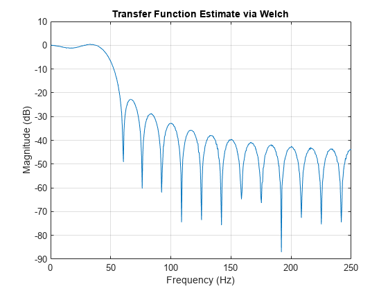
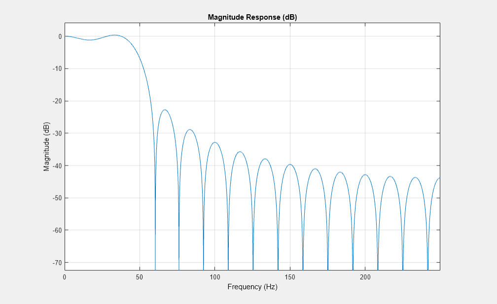
Se utiliza para verificar que la función de transferencia se aproxima a la respuesta de frecuencia del filtro.fvtool

fvtool(h,1,'Fs',fs)

Obtenga el mismo resultado devolviendo la estimación de la función de transferencia en una variable y trazando su valor absoluto en decibelios.

[Txy,f] = tfestimate(x,y,1024,[],[],fs);  plot(f,mag2db(abs(Txy)))

Función de transferencia SISO

Estime la función de transferencia para un sistema simple de entrada única/salida única y compárelo con la definición.

Un sistema oscilante unidimensional de tiempo discreto consiste en una unidad de masa,

<math display="inline">

<mrow>

<mi mathvariant="italic">m</mi>

</mrow>

</math>

, unida a una pared por un resorte de constante elástica unitaria. Un sensor muestrea la aceleración,

<math display="inline">

<mrow>

<mi mathvariant="italic">a</mi>

</mrow>

</math>

, de la Misa en

<math display="inline">

<mrow>

<msub>

<mrow>

<mi mathvariant="italic">F</mi>

</mrow>

<mrow>

<mi mathvariant="italic">s</mi>

</mrow>

</msub>

<mo stretchy="false">=</mo>

<mn>1</mn>

</mrow>

</math>

Hz. Un amortiguador impide el movimiento de la masa ejerciendo en ella una fuerza proporcional a la velocidad, con constante amortiguamiento

<math display="inline">

<mrow>

<mi mathvariant="italic">b</mi>

<mo stretchy="false">=</mo>

<mn>0</mn>

<mo stretchy="false">.</mo>

<mn>01</mn>

</mrow>

</math>

.

Genere 2000 muestras de tiempo. Defina el intervalo de muestreo

<math display="inline">

<mrow>

<mi>Δ</mi>

<mi mathvariant="italic">t</mi>

<mo>=</mo>

<mrow>

<mrow>

<mn>1</mn>

</mrow>

<mo>/</mo>

<mrow>

<msub>

<mrow>

<mi mathvariant="italic">F</mi>

</mrow>

<mrow>

<mi mathvariant="italic">s</mi>

</mrow>

</msub>

</mrow>

</mrow>

</mrow>

</math>

.

Fs = 1; dt = 1/Fs; N = 2000; t = dt*(0:N-1); b = 0.01;

El sistema puede describirse mediante el modelo de espacio de estado

<math display="block">

<mrow>

<mtable>

<mtr>

<mtd>

<mrow>

<mi>x</mi>

<mo stretchy="false">(</mo>

<mi>k</mi>

<mo>+</mo>

<mn>1</mn>

<mo stretchy="false">)</mo>

<mo>=</mo>

<mi>A</mi>

<mi>x</mi>

<mo stretchy="false">(</mo>

<mi>k</mi>

<mo stretchy="false">)</mo>

<mo>+</mo>

<mi>B</mi>

<mi>u</mi>

<mo stretchy="false">(</mo>

<mi>k</mi>

<mo stretchy="false">)</mo>

<mo>,</mo>

</mrow>

</mtd>

</mtr>

<mtr>

<mtd>

<mrow>

<mi>y</mi>

<mo stretchy="false">(</mo>

<mi>k</mi>

<mo stretchy="false">)</mo>

<mo>=</mo>

<mi>C</mi>

<mi>x</mi>

<mo stretchy="false">(</mo>

<mi>k</mi>

<mo stretchy="false">)</mo>

<mo>+</mo>

<mi>D</mi>

<mi>u</mi>

<mo stretchy="false">(</mo>

<mi>k</mi>

<mo stretchy="false">)</mo>

<mo>,</mo>

</mrow>

</mtd>

</mtr>

</mtable>

</mrow>

</math>

Dónde

<math display="inline">

<mrow>

<mi mathvariant="italic">x</mi>

<mo>=</mo>

<msup>

<mrow>

<mrow>

<mo>[</mo>

<mtable>

<mtr>

<mtd>

<mrow>

<mi mathvariant="italic">r</mi>

</mrow>

</mtd>

<mtd>

<mrow>

<mi mathvariant="italic">v</mi>

</mrow>

</mtd>

</mtr>

</mtable>

<mo>]</mo>

</mrow>

</mrow>

<mrow>

<mi mathvariant="italic">T</mi>

</mrow>

</msup>

</mrow>

</math>

es el vector del estado,

<math display="inline">

<mrow>

<mi mathvariant="italic">r</mi>

</mrow>

</math>

Y

<math display="inline">

<mrow>

<mi mathvariant="italic">v</mi>

</mrow>

</math>

son respectivamente la posición y la velocidad de la masa,

<math display="inline">

<mrow>

<mi mathvariant="italic">u</mi>

</mrow>

</math>

es la fuerza impulsora, y

<math display="inline">

<mrow>

<mi mathvariant="italic">y</mi>

<mo>=</mo>

<mi mathvariant="italic">a</mi>

</mrow>

</math>

es la salida medida. Las matrices de espacio de estado se

<math display="block">

<mrow>

<mi>A</mi>

<mo>=</mo>

<mi mathvariant="normal">exp</mi>

<mo stretchy="false">(</mo>

<msub>

<mrow>

<mi>A</mi>

</mrow>

<mrow>

<mi>c</mi>

</mrow>

</msub>

<mi>Δ</mi>

<mi>t</mi>

<mo stretchy="false">)</mo>

<mo>,</mo>

<mspace width="1em"></mspace>

<mi>B</mi>

<mo>=</mo>

<msubsup>

<mrow>

<mi>A</mi>

</mrow>

<mrow>

<mi>c</mi>

</mrow>

<mrow>

<mo>-</mo>

<mn>1</mn>

</mrow>

</msubsup>

<mo stretchy="false">(</mo>

<mi>A</mi>

<mo>-</mo>

<mi>I</mi>

<mo stretchy="false">)</mo>

<msub>

<mrow>

<mi>B</mi>

</mrow>

<mrow>

<mi>c</mi>

</mrow>

</msub>

<mo>,</mo>

<mspace width="1em"></mspace>

<mi>C</mi>

<mo>=</mo>

<mrow>

<mo>[</mo>

<mtable>

<mtr>

<mtd>

<mrow>

<mo>-</mo>

<mn>1</mn>

</mrow>

</mtd>

<mtd>

<mrow>

<mo>-</mo>

<mi>b</mi>

</mrow>

</mtd>

</mtr>

</mtable>

<mo>]</mo>

</mrow>

<mo>,</mo>

<mspace width="1em"></mspace>

<mi>D</mi>

<mo>=</mo>

<mn>1</mn>

<mo>,</mo>

</mrow>

</math>

<math display="inline">

<mrow>

<mi mathvariant="italic">I</mi>

</mrow>

</math>

es el

<math display="inline">

<mrow>

<mn>2</mn>

<mo>×</mo>

<mn>2</mn>

</mrow>

</math>

identidad y las matrices de espacio de estado de tiempo continuo se

<math display="block">

<mrow>

<msub>

<mrow>

<mi>A</mi>

</mrow>

<mrow>

<mi>c</mi>

</mrow>

</msub>

<mo>=</mo>

<mrow>

<mo>[</mo>

<mtable>

<mtr>

<mtd>

<mrow>

<mn>0</mn>

</mrow>

</mtd>

<mtd>

<mrow>

<mn>1</mn>

</mrow>

</mtd>

</mtr>

<mtr>

<mtd>

<mrow>

<mo>-</mo>

<mn>1</mn>

</mrow>

</mtd>

<mtd>

<mrow>

<mo>-</mo>

<mi>b</mi>

</mrow>

</mtd>

</mtr>

</mtable>

<mo>]</mo>

</mrow>

<mo>,</mo>

<mspace width="1em"></mspace>

<msub>

<mrow>

<mi>B</mi>

</mrow>

<mrow>

<mi>c</mi>

</mrow>

</msub>

<mo>=</mo>

<mrow>

<mo>[</mo>

<mtable>

<mtr>

<mtd>

<mrow>

<mn>0</mn>

</mrow>

</mtd>

</mtr>

<mtr>

<mtd>

<mrow>

<mn>1</mn>

</mrow>

</mtd>

</mtr>

</mtable>

<mo>]</mo>

</mrow>

<mo>.</mo>

</mrow>

</math>

Ac = [0 1;-1 -b]; A = expm(Ac*dt);  Bc = [0;1]; B = Ac\(A-eye(size(A)))*Bc;  C = [-1 -b]; D = 1;

La masa se impulsa por entrada aleatoria durante la mitad del intervalo de medición. Utilice el modelo de espacio de estado para calcular la evolución del tiempo del sistema a partir de un estado inicial de cero. Trazar la aceleración de la masa en función del tiempo.

rng default  u = zeros(1,N); u(1:N/2) = randn(1,N/2);  y = 0; x = [0;0]; for k = 1:N     y(k) = C*x + D*u(k);     x = A*x + B*u(k); end  plot(t,y)

Estimar la función de transferencia del sistema en función de la frecuencia. Utilice 2048 puntos DFT y especifique una ventana de Kaiser con un factor de forma de 15. Utilice el valor predeterminado de superposición entre los segmentos adyacentes.

nfs = 2048; wind = kaiser(N,15);  [txy,ft] = tfestimate(u,y,wind,[],nfs,Fs);

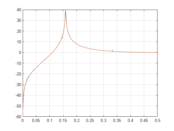
La función de respuesta de frecuencia de un sistema de tiempo discreto se puede expresar como la transformada Z de la función de transferencia de dominio de tiempo del sistema, evaluada en el círculo unitario. Compruebe que la estimación calculada coincide con esta definición.tfestimate

[b,a] = ss2tf(A,B,C,D);  fz = 0:1/nfs:1/2-1/nfs; z = exp(2j*pi*fz); frf = polyval(b,z)./polyval(a,z);  plot(ft,20*log10(abs(txy))) hold on plot(fz,20*log10(abs(frf))) hold off grid ylim([-60 40])

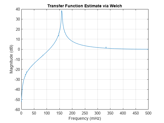
Trace la estimación utilizando la funcionalidad incorporada de.tfestimate

tfestimate(u,y,wind,[],nfs,Fs)

Función de transferencia del sistema MIMO

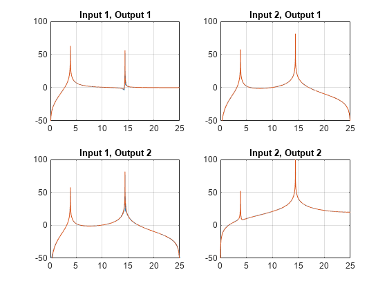
Estime la función de transferencia para un sistema simple de múltiples entradas/salidas múltiples.

Un sistema oscilante unidimensional ideal consta de dos masas,

<math display="inline">

<mrow>

<msub>

<mrow>

<mi mathvariant="italic">m</mi>

</mrow>

<mrow>

<mn>1</mn>

</mrow>

</msub>

</mrow>

</math>

Y

<math display="inline">

<mrow>

<msub>

<mrow>

<mi mathvariant="italic">m</mi>

</mrow>

<mrow>

<mn>2</mn>

</mrow>

</msub>

</mrow>

</math>

, confinado entre dos muros. Las unidades son tales que

<math display="inline">

<mrow>

<msub>

<mrow>

<mi mathvariant="italic">m</mi>

</mrow>

<mrow>

<mn>1</mn>

</mrow>

</msub>

<mo>=</mo>

<mn>1</mn>

</mrow>

</math>

Y

<math display="inline">

<mrow>

<msub>

<mrow>

<mi mathvariant="italic">m</mi>

</mrow>

<mrow>

<mn>2</mn>

</mrow>

</msub>

<mo>=</mo>

<mi>μ</mi>

</mrow>

</math>

. Cada masa se une a la pared más cercana por un resorte con una constante elástica

<math display="inline">

<mrow>

<mi mathvariant="italic">k</mi>

</mrow>

</math>

. Un resorte idéntico conecta las dos masas. Tres amortiguadores impiden el movimiento de las masas ejerciendo en ellas fuerzas proporcionales a la velocidad, con amortiguamiento constante

<math display="inline">

<mrow>

<mi mathvariant="italic">b</mi>

</mrow>

</math>

. La muestra de sensores

<math display="inline">

<mrow>

<msub>

<mrow>

<mi mathvariant="italic">a</mi>

</mrow>

<mrow>

<mn>1</mn>

</mrow>

</msub>

</mrow>

</math>

Y

<math display="inline">

<mrow>

<msub>

<mrow>

<mi mathvariant="italic">a</mi>

</mrow>

<mrow>

<mn>2</mn>

</mrow>

</msub>

</mrow>

</math>

, las aceleraciones de las masas, en

<math display="inline">

<mrow>

<msub>

<mrow>

<mi mathvariant="italic">F</mi>

</mrow>

<mrow>

<mi mathvariant="italic">s</mi>

</mrow>

</msub>

<mo>=</mo>

<mn>50</mn>

</mrow>

</math>

Hz.

Genere 30000 muestras de tiempo, equivalentes a 600 segundos. Defina el intervalo de muestreo

<math display="inline">

<mrow>

<mi>Δ</mi>

<mi mathvariant="italic">t</mi>

<mo>=</mo>

<mrow>

<mrow>

<mn>1</mn>

</mrow>

<mo>/</mo>

<mrow>

<msub>

<mrow>

<mi mathvariant="italic">F</mi>

</mrow>

<mrow>

<mi mathvariant="italic">s</mi>

</mrow>

</msub>

</mrow>

</mrow>

</mrow>

</math>

.

Fs = 50; dt = 1/Fs; N = 30000; t = dt*(0:N-1);

El sistema puede describirse mediante el modelo de espacio de estado

<math display="block">

<mrow>

<mtable>

<mtr>

<mtd>

<mrow>

<mi>x</mi>

<mo stretchy="false">(</mo>

<mi>k</mi>

<mo>+</mo>

<mn>1</mn>

<mo stretchy="false">)</mo>

<mo>=</mo>

<mi>A</mi>

<mi>x</mi>

<mo stretchy="false">(</mo>

<mi>k</mi>

<mo stretchy="false">)</mo>

<mo>+</mo>

<mi>B</mi>

<mi>u</mi>

<mo stretchy="false">(</mo>

<mi>k</mi>

<mo stretchy="false">)</mo>

<mo>,</mo>

</mrow>

</mtd>

</mtr>

<mtr>

<mtd>

<mrow>

<mi>y</mi>

<mo stretchy="false">(</mo>

<mi>k</mi>

<mo stretchy="false">)</mo>

<mo>=</mo>

<mi>C</mi>

<mi>x</mi>

<mo stretchy="false">(</mo>

<mi>k</mi>

<mo stretchy="false">)</mo>

<mo>+</mo>

<mi>D</mi>

<mi>u</mi>

<mo stretchy="false">(</mo>

<mi>k</mi>

<mo stretchy="false">)</mo>

<mo>,</mo>

</mrow>

</mtd>

</mtr>

</mtable>

</mrow>

</math>

Dónde

<math display="block">

<mrow>

<mi>x</mi>

<mo>=</mo>

<msup>

<mrow>

<mo>[</mo>

<mtable>

<mtr>

<mtd>

<mrow>

<msub>

<mrow>

<mi>r</mi>

</mrow>

<mrow>

<mn>1</mn>

</mrow>

</msub>

</mrow>

</mtd>

<mtd>

<mrow>

<msub>

<mrow>

<mi>v</mi>

</mrow>

<mrow>

<mn>1</mn>

</mrow>

</msub>

</mrow>

</mtd>

<mtd>

<mrow>

<msub>

<mrow>

<mi>r</mi>

</mrow>

<mrow>

<mn>2</mn>

</mrow>

</msub>

</mrow>

</mtd>

<mtd>

<mrow>

<msub>

<mrow>

<mi>v</mi>

</mrow>

<mrow>

<mn>2</mn>

</mrow>

</msub>

</mrow>

</mtd>

</mtr>

</mtable>

<mo>]</mo>

</mrow>

<mrow>

<mi>T</mi>

</mrow>

</msup>

</mrow>

</math>

es el vector del estado,

<math display="block">

<mrow>

<msub>

<mrow>

<mi>r</mi>

</mrow>

<mrow>

<mi>i</mi>

</mrow>

</msub>

</mrow>

</math>

Y

<math display="block">

<mrow>

<msub>

<mrow>

<mi>v</mi>

</mrow>

<mrow>

<mi>i</mi>

</mrow>

</msub>

</mrow>

</math>

son respectivamente la ubicación y la velocidad de la

<math display="block">

<mrow>

<mi>i</mi>

</mrow>

</math>

TH Mass,

<math display="block">

<mrow>

<mi>u</mi>

<mo>=</mo>

<msup>

<mrow>

<mo>[</mo>

<mtable>

<mtr>

<mtd>

<mrow>

<msub>

<mrow>

<mi>u</mi>

</mrow>

<mrow>

<mn>1</mn>

</mrow>

</msub>

</mrow>

</mtd>

<mtd>

<mrow>

<msub>

<mrow>

<mi>u</mi>

</mrow>

<mrow>

<mn>2</mn>

</mrow>

</msub>

</mrow>

</mtd>

</mtr>

</mtable>

<mo>]</mo>

</mrow>

<mrow>

<mi>T</mi>

</mrow>

</msup>

</mrow>

</math>

es el vector de las fuerzas impulsoras de entrada, y

<math display="block">

<mrow>

<mi>y</mi>

<mo>=</mo>

<msup>

<mrow>

<mo>[</mo>

<mtable>

<mtr>

<mtd>

<mrow>

<msub>

<mrow>

<mi>a</mi>

</mrow>

<mrow>

<mn>1</mn>

</mrow>

</msub>

</mrow>

</mtd>

<mtd>

<mrow>

<msub>

<mrow>

<mi>a</mi>

</mrow>

<mrow>

<mn>2</mn>

</mrow>

</msub>

</mrow>

</mtd>

</mtr>

</mtable>

<mo>]</mo>

</mrow>

<mrow>

<mi>T</mi>

</mrow>

</msup>

</mrow>

</math>

es el vector de salida. Las matrices de espacio de estado se

<math display="block">

<mrow>

<mi>A</mi>

<mo>=</mo>

<mi mathvariant="normal">exp</mi>

<mo stretchy="false">(</mo>

<msub>

<mrow>

<mi>A</mi>

</mrow>

<mrow>

<mi>c</mi>

</mrow>

</msub>

<mi>Δ</mi>

<mi>t</mi>

<mo stretchy="false">)</mo>

<mo>,</mo>

<mspace width="1em"></mspace>

<mi>B</mi>

<mo>=</mo>

<msubsup>

<mrow>

<mi>A</mi>

</mrow>

<mrow>

<mi>c</mi>

</mrow>

<mrow>

<mo>-</mo>

<mn>1</mn>

</mrow>

</msubsup>

<mo stretchy="false">(</mo>

<mi>A</mi>

<mo>-</mo>

<mi>I</mi>

<mo stretchy="false">)</mo>

<msub>

<mrow>

<mi>B</mi>

</mrow>

<mrow>

<mi>c</mi>

</mrow>

</msub>

<mo>,</mo>

<mspace width="1em"></mspace>

<mi>C</mi>

<mo>=</mo>

<mrow>

<mo>[</mo>

<mtable>

<mtr>

<mtd>

<mrow>

<mo>-</mo>

<mn>2</mn>

<mi>k</mi>

</mrow>

</mtd>

<mtd>

<mrow>

<mo>-</mo>

<mn>2</mn>

<mi>b</mi>

</mrow>

</mtd>

<mtd>

<mrow>

<mi>k</mi>

</mrow>

</mtd>

<mtd>

<mrow>

<mi>b</mi>

</mrow>

</mtd>

</mtr>

<mtr>

<mtd>

<mrow>

<mi>k</mi>

<mo>/</mo>

<mi>μ</mi>

</mrow>

</mtd>

<mtd>

<mrow>

<mi>b</mi>

<mo>/</mo>

<mi>μ</mi>

</mrow>

</mtd>

<mtd>

<mrow>

<mo>-</mo>

<mn>2</mn>

<mi>k</mi>

<mo>/</mo>

<mi>μ</mi>

</mrow>

</mtd>

<mtd>

<mrow>

<mo>-</mo>

<mn>2</mn>

<mi>b</mi>

<mo>/</mo>

<mi>μ</mi>

</mrow>

</mtd>

</mtr>

</mtable>

<mo>]</mo>

</mrow>

<mo>,</mo>

<mspace width="1em"></mspace>

<mi>D</mi>

<mo>=</mo>

<mrow>

<mo>[</mo>

<mtable>

<mtr>

<mtd>

<mrow>

<mn>1</mn>

</mrow>

</mtd>

<mtd>

<mrow>

<mn>0</mn>

</mrow>

</mtd>

</mtr>

<mtr>

<mtd>

<mrow>

<mn>0</mn>

</mrow>

</mtd>

<mtd>

<mrow>

<mn>1</mn>

<mo>/</mo>

<mi>μ</mi>

</mrow>

</mtd>

</mtr>

</mtable>

<mo>]</mo>

</mrow>

<mo>,</mo>

</mrow>

</math>

<math display="inline">

<mrow>

<mi mathvariant="italic">I</mi>

</mrow>

</math>

es el

<math display="inline">

<mrow>

<mn>4</mn>

<mo stretchy="false">×</mo>

<mn>4</mn>

</mrow>

</math>

identidad y las matrices de espacio de estado de tiempo continuo se

<math display="block">

<mrow>

<msub>

<mrow>

<mi>A</mi>

</mrow>

<mrow>

<mi>c</mi>

</mrow>

</msub>

<mo>=</mo>

<mrow>

<mo>[</mo>

<mtable>

<mtr>

<mtd>

<mrow>

<mn>0</mn>

</mrow>

</mtd>

<mtd>

<mrow>

<mn>1</mn>

</mrow>

</mtd>

<mtd>

<mrow>

<mn>0</mn>

</mrow>

</mtd>

<mtd>

<mrow>

<mn>0</mn>

</mrow>

</mtd>

</mtr>

<mtr>

<mtd>

<mrow>

<mo>-</mo>

<mn>2</mn>

<mi>k</mi>

</mrow>

</mtd>

<mtd>

<mrow>

<mo>-</mo>

<mn>2</mn>

<mi>b</mi>

</mrow>

</mtd>

<mtd>

<mrow>

<mi>k</mi>

</mrow>

</mtd>

<mtd>

<mrow>

<mi>b</mi>

</mrow>

</mtd>

</mtr>

<mtr>

<mtd>

<mrow>

<mn>0</mn>

</mrow>

</mtd>

<mtd>

<mrow>

<mn>0</mn>

</mrow>

</mtd>

<mtd>

<mrow>

<mn>0</mn>

</mrow>

</mtd>

<mtd>

<mrow>

<mn>1</mn>

</mrow>

</mtd>

</mtr>

<mtr>

<mtd>

<mrow>

<mi>k</mi>

<mo>/</mo>

<mi>μ</mi>

</mrow>

</mtd>

<mtd>

<mrow>

<mi>b</mi>

<mo>/</mo>

<mi>μ</mi>

</mrow>

</mtd>

<mtd>

<mrow>

<mo>-</mo>

<mn>2</mn>

<mi>k</mi>

<mo>/</mo>

<mi>μ</mi>

</mrow>

</mtd>

<mtd>

<mrow>

<mo>-</mo>

<mn>2</mn>

<mi>b</mi>

<mo>/</mo>

<mi>μ</mi>

</mrow>

</mtd>

</mtr>

</mtable>

<mo>]</mo>

</mrow>

<mo>,</mo>

<mspace width="1em"></mspace>

<msub>

<mrow>

<mi>B</mi>

</mrow>

<mrow>

<mi>c</mi>

</mrow>

</msub>

<mo>=</mo>

<mrow>

<mo>[</mo>

<mtable>

<mtr>

<mtd>

<mrow>

<mn>0</mn>

</mrow>

</mtd>

<mtd>

<mrow>

<mn>0</mn>

</mrow>

</mtd>

</mtr>

<mtr>

<mtd>

<mrow>

<mn>1</mn>

</mrow>

</mtd>

<mtd>

<mrow>

<mn>0</mn>

</mrow>

</mtd>

</mtr>

<mtr>

<mtd>

<mrow>

<mn>0</mn>

</mrow>

</mtd>

<mtd>

<mrow>

<mn>0</mn>

</mrow>

</mtd>

</mtr>

<mtr>

<mtd>

<mrow>

<mn>0</mn>

</mrow>

</mtd>

<mtd>

<mrow>

<mn>1</mn>

<mo>/</mo>

<mi>μ</mi>

</mrow>

</mtd>

</mtr>

</mtable>

<mo>]</mo>

</mrow>

<mo>.</mo>

</mrow>

</math>

Me

<math display="inline">

<mrow>

<mi mathvariant="italic">k</mi>

<mo>=</mo>

<mn>400</mn>

</mrow>

</math>

,

<math display="inline">

<mrow>

<mi mathvariant="italic">b</mi>

<mo stretchy="false">=</mo>

<mn>0</mn>

</mrow>

</math>

Y

<math display="inline">

<mrow>

<mi>μ</mi>

<mo>=</mo>

<mrow>

<mrow>

<mn>1</mn>

</mrow>

<mo>/</mo>

<mrow>

<mn>10</mn>

</mrow>

</mrow>

</mrow>

</math>

.

k = 400; b = 0; m = 1/10;  Ac = [0 1 0 0;-2*k -2*b k b;0 0 0 1;k/m b/m -2*k/m -2*b/m]; A = expm(Ac*dt); Bc = [0 0;1 0;0 0;0 1/m]; B = Ac\(A-eye(4))*Bc; C = [-2*k -2*b k b;k/m b/m -2*k/m -2*b/m]; D = [1 0;0 1/m];

Las masas son impulsadas por la entrada aleatoria a lo largo de la medición. Utilice el modelo de espacio de estado para calcular la evolución del tiempo del sistema a partir de un estado inicial de cero.

rng default u = randn(2,N);  x = [0;0;0;0]; for kk = 1:N     y(:,kk) = C*x + D*u(:,kk);     x = A*x + B*u(:,kk); end

Utilice los datos de entrada y salida para estimar la función de transferencia del sistema en función de la frecuencia. Especifique la opción para producir las cuatro funciones de transferencia.'mimo' Utilice una ventana Hann de 5000 muestras para dividir las señales en segmentos. Especifique 2500 muestras de superposición entre segmentos adyacentes y

<math display="inline">

<mrow>

<msup>

<mrow>

<mn>2</mn>

</mrow>

<mrow>

<mn>14</mn>

</mrow>

</msup>

</mrow>

</math>

Puntos DFT. Trace las estimaciones.

wind = hann(5000); nov = 2500;  [q,fq] = tfestimate(u',y',wind,nov,2^14,Fs,'mimo');

Calcule la función de transferencia teórica como la transformación Z de la función de transferencia de dominio de tiempo, evaluada en el círculo de la unidad.

nfs = 2^14;  fz = 0:1/nfs:1/2-1/nfs; z = exp(2j*pi*fz);  [b1,a1] = ss2tf(A,B,C,D,1); [b2,a2] = ss2tf(A,B,C,D,2);  frf(1,:,1) = polyval(b1(1,:),z)./polyval(a1,z); frf(1,:,2) = polyval(b1(2,:),z)./polyval(a1,z);  frf(2,:,1) = polyval(b2(1,:),z)./polyval(a2,z); frf(2,:,2) = polyval(b2(2,:),z)./polyval(a2,z);

Trazar las funciones teóricas de transferencia y sus correspondientes estimaciones.

for jk = 1:2     for kj = 1:2         subplot(2,2,2*(jk-1)+kj)         plot(fq,20*log10(abs(q(:,jk,kj))))         hold on         plot(fz*Fs,20*log10(abs(frf(jk,:,kj))))         hold off         grid         title(['Input ' int2str(kj) ', Output ' int2str(jk)])         axis([0 Fs/2 -50 100])     end end

Las funciones de transferencia tienen máximos en los valores esperados,

<math display="inline">

<mrow>

<mrow>

<mrow>

<msub>

<mrow>

<mi>ω</mi>

</mrow>

<mrow>

<mn>1</mn>

<mo>,</mo>

<mn>2</mn>

</mrow>

</msub>

</mrow>

<mo>/</mo>

<mrow>

<mn>2</mn>

<mi>π</mi>

</mrow>

</mrow>

</mrow>

</math>

, donde el

<math display="inline">

<mrow>

<mi>ω</mi>

</mrow>

</math>

son los valores propios de la matriz modal.

sqrt(eig(k*[2 -1;-1/m 2/m]))/(2*pi)

ans = 2×1

    3.8470
   14.4259

Añada amortiguación al sistema estableciendo

<math display="inline">

<mrow>

<mi mathvariant="italic">b</mi>

<mo>=</mo>

<mn>0</mn>

<mo>.</mo>

<mn>1</mn>

</mrow>

</math>

. Calcule la evolución del tiempo del sistema amortiguado con las mismas fuerzas de conducción. Calcule el

<math display="inline">

<mrow>

<msub>

<mrow>

<mi mathvariant="italic">H</mi>

</mrow>

<mrow>

<mn>2</mn>

</mrow>

</msub>

</mrow>

</math>

estimación de la función de transferencia MIMO utilizando la misma ventana y solapamiento. Trace las estimaciones utilizando la funcionalidad.tfestimate

b = 0.1;  Ac = [0 1 0 0;-2*k -2*b k b;0 0 0 1;k/m b/m -2*k/m -2*b/m]; A = expm(Ac*dt); B = Ac\(A-eye(4))*Bc; C = [-2*k -2*b k b;k/m b/m -2*k/m -2*b/m];  x = [0;0;0;0]; for kk = 1:N     y(:,kk) = C*x + D*u(:,kk);     x = A*x + B*u(:,kk); end  clf tfestimate(u',y',wind,nov,[],Fs,'mimo','Estimator','H2') legend('I1, O1','I1, O2','I2, O1','I2, O2')

yl = ylim;

Compare las estimaciones con las predicciones teóricas.

[b1,a1] = ss2tf(A,B,C,D,1); [b2,a2] = ss2tf(A,B,C,D,2);  frf(1,:,1) = polyval(b1(1,:),z)./polyval(a1,z); frf(1,:,2) = polyval(b1(2,:),z)./polyval(a1,z);  frf(2,:,1) = polyval(b2(1,:),z)./polyval(a2,z); frf(2,:,2) = polyval(b2(2,:),z)./polyval(a2,z);  plot(fz*Fs,20*log10(abs(reshape(permute(frf,[2 1 3]),[nfs/2 4])))) legend('I1, O1','I1, O2','I2, O1','I2, O2') ylim(yl) grid

Argumentos de entrada

x — Señal de entrada

Vector | Matriz

Señal de entrada, especificada como vector o matriz.

Ejemplo: especifica una sinusoide incrustada en el ruido Gaussiano blanco.cos(pi/4*(0:159))+randn(1,160)

Tipos de datos: single | double
Soporte de números complejos: Sí

y — Señal de salida

Vector | Matriz

Señal de salida, especificada como vector o matriz.

Tipos de datos: single | double
Soporte de números complejos: Sí

window — Ventana

Entero | Vector | []

Window, especificado como un entero o como un vector de fila o columna. Se utiliza para dividir la señal en segmentos.window

• Si es un número entero, a continuación, divide y en segmentos de longitud y ventanas de cada segmento con una ventana de Hamming de esa longitud.windowtfestimatexywindow

• Si es un vector, a continuación, divide y en segmentos de la misma longitud que el vector y ventanas de cada segmento utilizando.windowtfestimatexywindow

Si la longitud de y no se puede dividir exactamente en un número entero de segmentos con muestras superpuestas, las señales se truncan en consecuencia.xynoverlap

Si especifica como vacío, a continuación, utiliza una ventana de Hamming tal que y se dividen en ocho segmentos con muestras superpuestas.windowtfestimatexynoverlap

Para obtener una lista de las ventanas disponibles, consulte.Windows

Ejemplo: y ambos especifican una ventana Hann de longitud + 1.hann(N+1)(1-cos(2*pi*(0:N)'/N))/2N

Tipos de datos: single | double

noverlap — Número de muestras superpuestas

entero positivo | []

Número de muestras superpuestas, especificadas como un entero positivo.

• Si es escalar, debe ser menor que.windownoverlapwindow

• Si es un vector, debe ser menor que la longitud de.windownoverlapwindow

Si especifica como vacío, utiliza un número que produce una superposición del 50% entre los segmentos.noverlaptfestimate Si la longitud del segmento no está especificada, la función se establece en ⌊/4,5 ⌋, donde es la longitud de las señales de entrada y salida.noverlapNN

Tipos de datos: double | single

nfft — Número de puntos DFT

entero positivo | []

Número de puntos DFT, especificado como un entero positivo. Si especifica como vacío, a continuación, establece este argumento paranffttfestimate max(256,2^p)Dónde p = ⌈log₂ N⌉ para las señales de entrada de longitud.N

Tipos de datos: single | double

fs — Frecuencia de muestreo

escalar positivo

Frecuencia de muestreo, especificada como un escalar positivo. La frecuencia de muestreo es el número de muestras por unidad de tiempo. Si la unidad de tiempo es de segundos, entonces la frecuencia de muestreo tiene unidades de Hz.

w — Las frecuencias normalizadas

Vector

Frecuencias normalizadas, especificadas como un vector de fila o columna con al menos dos elementos. Las frecuencias normalizadas están en Rad/sample.

Ejemplo: w = [pi/4 pi/2]

Tipos de datos: double

f — Frecuencias

Vector

Frecuencias, especificadas como un vector de fila o columna con al menos dos elementos. Las frecuencias están en ciclos por unidad de tiempo. La hora de la unidad se especifica mediante la frecuencia de muestreo,.fs Si tiene unidades de muestras/segundo, entonces tiene unidades de Hz.fsf

Ejemplo: fs = 1000; f = [100 200]

Tipos de datos: double

freqrange — Rango de frecuencias para la estimación de función de transferencia

'onesided' | 'twosided' | 'centered'

Rango de frecuencias para la estimación de la función de transferencia, especificada como una de, o.'onesided''twosided''centered' El valor predeterminado es para las señales con valores reales y para las señales con valores complejos.'onesided''twosided'

• : Devuelve la estimación unilateral de la función de transferencia entre dos señales de entrada con valores reales y.'onesided'xy Si es Even, tiene/2 + 1 filas y se calcula en el intervalonffttxynfft [0,π] RAD/sample. Si es impar, tiene (+ 1)/2 filas y el intervalo esnffttxynfft [0,π) RAD/sample. Si se especifica, los intervalos correspondientes son [0,/2] ciclos/unidad de tiempo para pares y [0,/2) ciclos/unidad de tiempo para impar.fsfsnfftfsnfft

• : Devuelve la estimación bilateral de la función de transferencia entre dos señales de entrada con valores complejos o de valor real, y.'twosided'xy En este caso, tiene filas y se calcula a lo largo del intervalotxynfft [0,2π) RAD/sample. Si se especifica, el intervalo es [0,) ciclos/unidad de tiempo.fsfs

• : Devuelve la estimación centrada a dos caras de la función de transferencia entre dos señales de entrada con valores complejos o de valor real, y.'centered'xy En este caso, tiene filas y se calcula a lo largo del intervalotxynfft (–π,π] RAD/sample para Even ynfft (–π,π) RAD/sample para Odd.nfft Si especifica, los intervalos correspondientes son (–/2,/2] ciclos/unidad de tiempo para pares y (–/2,/2) ciclos/unidad de tiempo para impar.fsfsfsnfftfsfsnfft

est — Calculadora de función de transferencia

'H1' (predeterminado) | 'H2'

Calculadora de función de transferencia, especificada como o.'H1''H2'

• Utilíla cuando el ruido no esté correlacionado con las señales de entrada.'H1'

• Se utiliza cuando el ruido no está correlacionado con las señales de salida.'H2' En este caso, el número de señales de entrada debe ser igual al número de señales de salida.

Consulte para obtener más información.Función de transferencia

Argumentos de salida

txy — La estimación de función de transferencia

Vector | Matriz | matriz tridimensional

Estimación de la función de transferencia, devuelta como vector, matriz o matriz tridimensional.

w — Las frecuencias normalizadas

Vector

Frecuencias normalizadas, devueltas como un vector de columna de valor real.

f — Las frecuencias cíclicas

Vector

Frecuencias cíclicas, devueltas como un vector de columna de valor real.

Más acerca de

Función de transferencia

La relación entre la entrada y la salida está modelada por el lineal, invariable de tiempo.xytransfer functiontxy En el dominio de frecuencia, Y(f) = H(f)X(f).

• Para un único sistema de entrada/salida única, el H₁ estimación de la función de transferencia viene dada por

  $$H_1(f)=\frac{P_{yx}\left(f\right)}{P_{xx}\left(f\right)},$$

  Dónde P_yx es la densidad espectral de potencia cruzada de y, yxy P_xx es la densidad espectral de potencia de.x Esta estimación presupone que el ruido no está correlacionado con la entrada del sistema.

  Para sistemas de entrada múltiple/múltiples salidas (MIMO), el H₁ estimador se convierte en

  $$H_1(f)=P_{YX}(f)P_{XX}^{-1}(f)=\left[\begin{array}{cccc}{P}_{y_1{x}_1}(f)& P_{y_1{x}_2}(f)& \cdots & P_{y_1{x}_m}(f)\\ P_{y_2{x}_1}(f)& P_{y_2{x}_2}(f)& \cdots & P_{y_2{x}_m}(f)\\ ⋮& ⋮& \ddots & ⋮\\ P_{y_n{x}_1}(f)& P_{y_n{x}_2}(f)& \cdots & P_{y_n{x}_m}(f)\end{array}\right]{\left[\begin{array}{cccc}{P}_{x_1{x}_1}(f)& P_{x_1{x}_2}(f)& \cdots & P_{x_1{x}_m}(f)\\ P_{x_2{x}_1}(f)& P_{x_2{x}_2}(f)& \cdots & P_{x_2{x}_m}(f)\\ ⋮& ⋮& \ddots & ⋮\\ P_{x_m{x}_1}(f)& P_{x_m{x}_2}(f)& \cdots & P_{x_m{x}_m}(f)\end{array}\right]}^{-1}$$

  para entradas y salidas, donde:mn

  • P_yixk es la densidad espectral de potencia cruzada de la entrada TH y la salida TH.ki

  • P_xixk es la densidad espectral de potencia cruzada de las entradas TH y TH.ki

  Para dos entradas y dos salidas, el estimador es la matriz

  $$H_1(f)=\frac{\left[\begin{array}{cc}{P}_{y_1{x}_1}(f)P_{x_2{x}_2}(f)-P_{y_1{x}_2}(f)P_{x_2{x}_1}(f)& P_{y_1{x}_2}(f)P_{x_1{x}_1}(f)-P_{y_1{x}_1}(f)P_{x_1{x}_2}(f)\\ P_{y_2{x}_1}(f)P_{x_2{x}_2}(f)-P_{y_2{x}_2}(f)P_{x_2{x}_1}(f)& P_{y_2{x}_2}(f)P_{x_1{x}_1}(f)-P_{y_2{x}_1}(f)P_{x_1{x}_2}(f)\end{array}\right]}{P_{x_1{x}_1}(f)P_{x_2{x}_2}(f)-P_{x_1{x}_2}(f)P_{x_2{x}_1}(f)}.$$

• Para un único sistema de entrada/salida única, el H₂ estimación de la función de transferencia viene dada por

  $$H_2\left(f\right)=\frac{P_{yy}\left(f\right)}{P_{xy}\left(f\right)},$$

  Dónde P_yy es la densidad espectral de potencia de yy P_xy = P^*_yx es el conjugada compleja de la densidad espectral de potencia cruzada de y.xy Esta estimación asume que el ruido no está correlacionado con la salida del sistema.

  Para los sistemas MIMO, el H₂ estimador está bien definido sólo para el mismo número de entradas y salidas: n = m. El estimador se convierte en

  $$H_2(f)=P_{YY}(f)P_{XY}^{-1}(f)=\left[\begin{array}{cccc}{P}_{y_1{y}_1}(f)& P_{y_1{y}_2}(f)& \cdots & P_{y_1{y}_n}(f)\\ P_{y_2{y}_1}(f)& P_{y_2{y}_2}(f)& \cdots & P_{y_2{y}_n}(f)\\ ⋮& ⋮& \ddots & ⋮\\ P_{y_n{y}_1}(f)& P_{y_n{y}_2}(f)& \cdots & P_{y_n{y}_n}(f)\end{array}\right]{\left[\begin{array}{cccc}{P}_{x_1{y}_1}(f)& P_{x_1{y}_2}(f)& \cdots & P_{x_1{y}_n}(f)\\ P_{x_2{y}_1}(f)& P_{x_2{y}_2}(f)& \cdots & P_{x_2{y}_n}(f)\\ ⋮& ⋮& \ddots & ⋮\\ P_{x_n{y}_1}(f)& P_{x_n{y}_2}(f)& \cdots & P_{x_n{y}_n}(f)\end{array}\right]}^{-1},$$

  Dónde:

  • P_yiyk es la densidad espectral de potencia cruzada de las salidas TH y TH.ki

  • P_xiyk es el conjugada compleja de la densidad espectral de potencia cruzada de la entrada TH y la salida TH.ik

Algoritmos

utiliza el método de periodograma promediado de Welch.tfestimate Ver para más detalles.pwelch

Referencias

[1] Vold, Håvard, John Crowley, and G. Thomas Rocklin. “New Ways of Estimating Frequency Response Functions.” Sound and Vibration. Vol. 18, November 1984, pp. 34–38.

Consulte también

cpsd | mscohere | periodogram | pwelch

Introducido antes de R2006a

×

Open Example (es)

A modified version of this example exists on your system. Do you want to open this version instead? (es)

No, overwrite the modified version (es) Yes (es)