Determine Step Size
For the first step in Model Preparation Process, you obtain results from a variable-step simulation of the reference version of your Simscape™ model. The reference results provide a baseline against which you can assess the accuracy of your model as you modify it. This example shows how to analyze the reference results and the step size that the variable-step solver takes to:
Estimate the maximum step size that you can use for a fixed-step simulation
Identify events that have the potential to limit the maximum step size
Discontinuities and rapid changes require small step sizes for accurately capturing these dynamics. The maximum step size that you can use for a fixed-step simulation must be small enough to ensure accurate results. If your model contains such dynamics, then it is possible that the required step size for accurate results, Tsmax, is too small. A step size that is too small does not allow your real-time computer to finish calculating the solution for any given step in the simulation.
The analysis in this example helps you to estimate the maximum step size that fixed-step solvers can use and still obtain accurate results. You can also use the analysis to determine which elements influence the maximum step size for accurate results.
To open the reference model, at the MATLAB® command prompt, enter:
model = 'ssc_pneumatic_rts_reference';
open_system(model)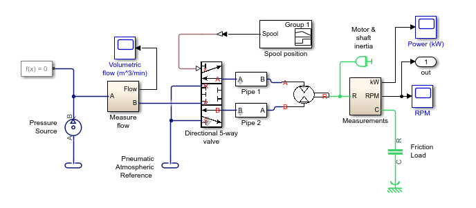
Simulate the model:
sim(model)
Create a semilogarithmic plot that shows how the step size for the solver varies during the simulation.
h1 = figure;
semilogy(tout(1:end-1),diff(tout),'-x')
title('Solver Step Size')
xlabel('Time (s)')
ylabel('Step Size (s)')
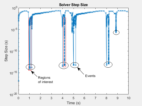
For much of the simulation, the step size is greater than the value of the Tsmax in the plot. The corresponding value, ~0.001 seconds, is an estimated maximum step size for achieving accurate results during fixed-step simulation with the model. To see how to configure the step size for fixed-step solvers for real-time simulation, see Choose Step Size and Number of Iterations.
The
xmarkers in the plot indicate the time that the solver took to execute a single step at that moment in the simulation. The step-size data is discrete. The line that connects the discrete points exists only to help you see the order of the individual execution times over the course of the simulation.A large decrease in step size indicates that the solver detects a zero-crossing event. Zero-crossing detection can happen when the value of a signal changes sign or crosses a threshold. The simulation reduces the step size to capture the dynamics for the zero-crossing event accurately. After the solver processes the dynamics for a zero-crossing event, the simulation step size can increase. It is possible for the solver to take several small steps before returning to the step size that precedes the zero-crossing event. The areas in the red boxes contain variations in recovery time for the variable step solver.
To see different post-zero-crossing behaviors, zoom to the region in the red box at time (t) = ~1 second.
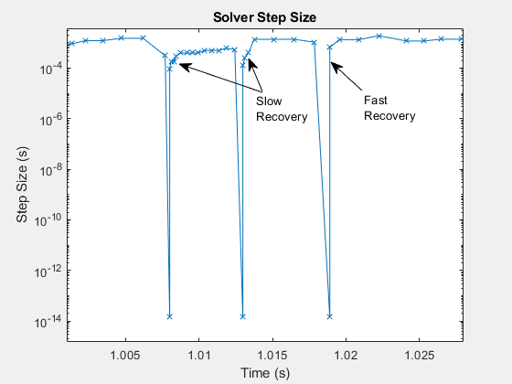
After t = 1.005 seconds, the step size decreases from ~10e-3 seconds to less than 10e-13 seconds to capture an event. The step size increases quickly to ~10e-5 seconds, and then slowly to ~10e-4 seconds. The step size decreases to capture a second event and recovers quickly, and then slowly to the step size from before the first event. The slow rates of recovery indicate that the simulation is using small steps to capture the dynamics of elements in your model. If the required step size limits the maximum fixed-step size to a small enough value, then an overrun might occur when you attempt simulation on your real-time computer.
The types of elements that require small step size are:
Elements that cause discontinuities, such as hard-stops and stick-slip friction
Elements that have small time constants, such as small masses with undamped, stiff springs and hydraulic circuits with small, compressible volumes
The step size recovers more quickly after it slows down to process the event that occurs before t = 1.02 seconds. This event is less likely to require small step sizes to achieve accurate results.
To see different types of slow solver recoveries, zoom to the region within the red box at t = ~4.2 seconds.
h1;
xZoomStart2 = 4.16;
xZoomEnd2 = 4.24;
yZoomStart2 = 10e-20;
yZoomEnd2 = 10e-1;
axis([xZoomStart2 xZoomEnd2 yZoomStart2 yZoomEnd2]);
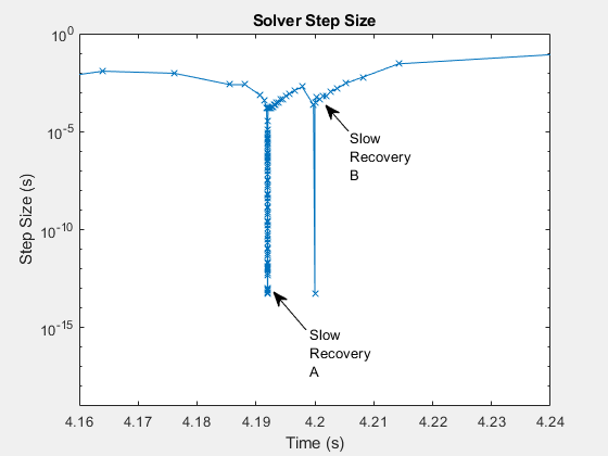
Just as there are different types of events that cause solvers to slow down, there are different types of slow solver recovery. The events that occur just before t = 4.19 and 4.2 seconds both involve zero-crossings. The solver takes a series of progressively larger steps as it reaches the step size from before the event. The large number of very small steps that follow the zero crossing at Slow Recovery A indicate that the element that caused the zero crossing is also numerically stiff.
The quicker step-size increase after the event that occurs at t = 4.2 seconds indicates that the element that caused the zero crossing before Slow Recovery B, is not as stiff as the event at Slow Recovery A.
To see the results, open the Simscape Results Explorer.
sscexplore(simlog)
Examine the angular speed. In the Simscape Results Explorer window, in the simulation log tree hierarchy, select Measurements > Ideal Rotational Motion Sensor >
 w.
w.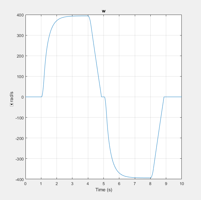
To add a plot of the gas flow, select Measure Flow > Pneumatic Mass & Heat Flow Sensor and then, use Ctrl+click to select
G_ps.
The slow recovery times occur when the simulation initializes, and approximately at t = 1, 4, 5, 8, and 9 seconds. These periods of small steps coincide with these times:
The motor speed is near zero rpm (simulation time t = ~ 1, 5, and 9 seconds)
The step change in motor speed is initiated from a steady-state speed to a new speed (time t = ~ 4 and 8 seconds)
The step change in flow rate is initiated from a steady-state speed to a new flow rate (time t = ~ 4 and 8 seconds)
The volumetric flow rate is near zero kg/s (t = ~ 1, 4, and 5 seconds)
These results indicate that the slow step-size recoveries are most likely due to elements in the model that involve friction or that have small, compressible volumes. To see how to identify the problematic elements and modify them to increase simulation speed, see Reduce Numerical Stiffness and Reduce Zero Crossings.