Configure Model Linearization Options

This topic shows how to configure linearization options when interactively linearizing models using the Model Linearizer app. For information on configuring options for programmatic linearization, see linearizeOptions.

To configure linearization options in Model Linearizer, on the Linear Analysis tab, click More Options.

Then, in the Options for exact linearization dialog box, specify your linearization settings.

For more information on specifying the order of the states in your linearized model, see Order States in Linearized Model.

Specify Model Sample Time

To specify the sample time of the final linearized model, use the Sample time parameter. You can specify the following sample time values.

• -1 — Set the sample time to the least common multiple of the nonzero sample times in the model.

• 0 — Create a continuous-time model.

• Positive scalar — Specify the sample time in seconds for discrete-time systems.

Select Linearization Algorithm

To specify the linearization algorithm, use the Choose algorithm drop-down list. You can select one of the following linearization algorithms.

• Block-by-block analytic — Individually linearize each block in the model, and combine the results to produce the linearization of the specified system.

• Numerical perturbation (forward difference) — Full-model numerical-perturbation linearization in which root-level inports and states are perturbed using forward differences; that is, by adding perturbations to the input and state values. This perturbation method is typically faster than the Numerical perturbation (central difference) method.

• Numerical perturbation (central difference) — Full-model numerical-perturbation linearization in which root-level inports and states are numerically perturbed using central differences; that is, by perturbing the input and state values in both positive and negative directions. This perturbation method is typically more accurate than the Numerical perturbation (forward difference) method.

The numerical perturbation linearization methods ignore linear analysis points set in the model and use root-level inports and outports instead.

Block-by-block linearization has several advantages over full-model numerical perturbation:

• Many Simulink^® blocks have a preprogrammed exact linearization.

• You can use linear analysis points to specify a portion of the model to linearize.

• You can configure blocks to use custom linearizations without affecting your model simulation.

• Structurally nonminimal states are automatically removed.

• You can specify linearizations that include uncertainty (requires Robust Control Toolbox™ software).

• You can obtain detailed diagnostic information about the linearization.

For more information on block-by-block linearization settings, see Block-by-Block Settings.

For more information on numerical perturbation linearization settings, see Numerical Perturbation Settings.

Store Offsets with Linear Model

To compute linearization offsets that correspond to the operating point at which the model was linearized, select Store offsets with linear model. The computed offsets are stored in the resulting linearized model object.

The software computes offsets for model inputs, outputs, states, and state derivatives. For more information, see the Offsets property of the ss model object.

Block-by-Block Settings

When you select the Block-by-block analytic linearization method, configure the linearization algorithm using the following settings.

Block Reduction Scope

Since R2025a

You can exclude nonminimal states from your linear model using the Block reduction scope parameter. Nonminimal states include states in blocks that are not on the linearization path; that is, blocks that lie on signal paths containing any of the following:

• Signals marked as open-loop linear analysis points

• Blocks that linearize to zero

• Switch blocks that are not active along the path

• Disabled subsystems

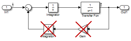
For example, the linearization result of the model shown in the following figure includes only states from the Integrator and Transfer Fcn blocks. The linear model excludes other blocks because they lie on a linearization path that includes a block that linearizes to zero (the zero gain block).

You can specify the following values for block reduction:

• None — Do not remove any nonminimal states.

• Full — Remove all nonminimal states not on the linearization path. For batch linearization applications, this option can produce inconsistent state definitions across the resulting linear models.

• Consistent across models — Remove only states that are not on the linearization path for all models in a batch linearization result. If you are generating a single linear model,this option is equivalent to selecting Full.

Before R2025a: Select the Exclude non-minimal states from linear models using block reduction parameter to exclude nonminimal states from your model. To include all states. clear this parameter. In this case, the software excludes all nonminimal states from all batch linearization results.

Exclude Discrete States from Linear Models

Select Exclude discrete states from linear models to exclude any discrete states from the linearization and accept the D-matrix value for all blocks with discrete states. You can use this option when you perform continuous linearizations (sample time set to 0) with the block-by-block analytic algorithm.

Clear this parameter to include discrete states in the linearization. Discrete states convert to continuous states using the rate conversion method you specify.

Return Linear Model with Exact Delays

Select Return linear model with exact delays to return a linear model with exact delay representations. You can use this parameter when you perform block-by-block analytic linearization of models with time delays.

Clear this parameter to return a linear model with Padé approximations of delays as specified in your Transport Delay and Variable Transport Delay blocks.

For more information on linearizing models with delays, see Models with Time Delays.

Recompile Model When Varying Parameter Values

By default, Model Linearizer computes all linearizations with a single compilation whenever it is possible to do so. In this case:

• If all varying parameters are tunable, linearizations are computed for all parameter-grid points with a single compilation.

• If some varying parameters are not tunable, the model is recompiled for each parameter-grid point, and the software issues a warning.

Select Recompile model when varying parameter values to force Model Linearizer to recompile the model for each point in the parameter grid.

Suppose that you are performing batch linearization by varying the values of tunable parameters and notice that the software is recompiling the model more than necessary. To ensure that linearizations are computed with a single compilation whenever possible, make sure that Recompile model when varying parameter values is cleared.

For more information about model compilation when you linearize with parameter variation, see Batch Linearization Efficiency When You Vary Parameter Values.

Rate Conversion Options

Changing the rate conversion method changes the way in which the software linearizes models containing several different sample rates. When you linearize a multirate system, you can set the Choose rate conversion method option to one of the following rate conversion methods.

• Zero-Order Hold — Use use the zero-order hold rate conversion method

• Tustin — Use the Tustin (bilinear) approximation

• Tustin with Prewarping — Use the Tustin approximation with prewarping

• Upsample when possible, Zero-Order Hold otherwise — Upsample discrete states when possible and use zero-order hold otherwise

• Upsample when possible, Tustin otherwise — Upsample discrete states when possible and use a Tustin approximation otherwise

• Upsample when possible, Tustin with Prewarping otherwise — Upsample discrete states when possible and use Tustin with prewarping otherwise

When you select Tustin with Prewarping or Upsample when possible, Tustin with Prewarping otherwise, set the Prewarp frequency option to the desired prewarp frequency in rad/s.

For more information on methods and algorithms for rate conversions and linearization of multirate models, see:

• Linearize Multirate Models

• Linearize Models Using Different Rate Conversion Methods

• Continuous-Discrete Conversion Methods

Note

You can only upsample when you convert discrete states to a new sample time that is an integer-value-times faster than the sampling time of the original system.

Numerical Perturbation Settings

The Relative perturbation level, State perturbation level, and Input perturbation level parameters set the perturbation levels for the numerical perturbation linearization algorithms. To set these fields, first select Numerical perturbation (forward difference) or Numerical perturbation (central difference) as the Linearization algorithm.

For more information on the numerical perturbation algorithms, see Perturbation of Individual Blocks.

The Relative perturbation level parameter sets the perturbation levels for both the states and the inputs of a model, according to the formula below, unless perturbation levels for the states or inputs are individually set in the State perturbation level or Input perturbation level fields.

When you set the Relative perturbation level value, P, the numerical perturbation linearization algorithms computes the perturbation of each state according to the following formula

$$P+\left(1e-3\right)\times P\times \left|x\right|$$

where x is a vector of the operating point values for the states in the model.

Similarly, the perturbation of the system's inputs is specified by

$$P+\left(1e-3\right)\times P\times \left|u\right|$$

where u is a vector of the operating point values for the inputs in the model.

Note that the relative perturbation of a state or input consists of both an absolute part and a relative part. Both parts use the Relative perturbation level value, P.

Alternatively, you can set the absolute perturbation levels for the states or inputs in your system using the State perturbation level or Input perturbation level parameter, respectively. These values override the state perturbations that are computed from the Relative perturbation level value.

To perturb all states or all inputs by the same amounts, set the corresponding parameter to a scalar value. To specify perturbation levels for each state or each input, set the corresponding parameter to an operating point object (created using operpoint) that contains the absolute perturbation values.

Label Channels and States with Full Block Path

Use the Label input/output channels and states with full block path parameter to specify how the names of states, and linearization inputs and outputs (I/O) appear in the

• Linearization results in Model Linearizer

• Title and data markers on linear model response plots in Linear System Analyzer

To show only state and I/O names, clear this parameter. Use this option when the signal names are unique and you know their locations in your Simulink model.

To show state and I/O names with full path in the model, select this parameter.

Label Channels with Bus Signal Names

Use the Label input/output channels with bus signal names parameter to specify how to label signals associated with linearization I/O points on bus signals in the linear model (applies only when you select an entire bus as an I/O point).

Selecting an entire bus signal is not recommended. Instead, select individual bus elements to:

• Obtain the linearization only for the channels that you are interested in

• Specify multiple I/Os, possibly as different types, in the same bus

To label I/Os on bus signals using the bus signal channel number, clear this parameter.

To label I/Os on bus signals using the signal names of the individual bus elements, select this parameter.

Bus signal names appear when the I/O points appear at the output point of the following blocks:

• Root-level inport block containing a bus object

• Bus creator block

• Subsystem block whose source traces back to one of the following places:

  • Output of a bus creator block

  • Root-level inport block by passing through only virtual or nonvirtual subsystem boundaries