Dynamics Analysis of a Robotic Arm in MATLAB

This example demonstrates a workflow for dynamics analysis of a serial link robotic arm in MATLAB® using Simscape™ Multibody™. It demonstrates various classes under simscape.multibody.* namespace to build and analyze a multibody system in MATLAB.

The example shows how to:

1. Build a serial link robotic system programmatically.

2. Generate a user-defined end-effector path.

3. Solve inverse kinematics involving joint limits via optimization to find joint positions.

4. Generate joint trajectories subject to kinematic constraints.

5. Use a root-finding approach to compute the maximum lifting force such that at least one joint actuator reaches its torque limit.

Build a Robotic Arm

Build a serial link robotic arm. The buildSerialLinkManipulator function constructs a Multibody model in the workspace, which is then compiled to obtain a CompiledMultibody (cmb):

% To simplify the process and avoid repeatedly typing the namespace name
% for the classes, you can use the import function.
import simscape.Value simscape.op.* simscape.multibody.*;
addpath(fullfile('DynamicsAnalysisOfARoboticArmInMATLABSupport','Scripts'));

mb = buildSerialLinkManipulator;
cmb = compile(mb);

Generate an End-Effector Path

Define a smooth arc from a start position to an end position for the end-effector of the robotic arm. The arc should reach its maximum height in the z-axis at the midpoint:

numIterations = 25;                % Number of discrete points along the trajectory
startPos = [0.5, 0,   0];          % [x, y, z] start
endPos   = [0,   0.5, 0];          % [x, y, z] end
zPeak    = 0.5;                    % Maximum z-height at the arc midpoint

s = linspace(0, 1, numIterations); % Parameter s in [0..1], for numIterations points
tVals = 3*s.^2 - 2*s.^3;           % Smooth step function t(s) = 3s^2 - 2s^3

% Compute X & Y via linear interpolation between start and end
x = startPos(1) + (endPos(1) - startPos(1)).*tVals;
y = startPos(2) + (endPos(2) - startPos(2)).*tVals;

% Sine bump in Z from 0 up to zPeak, back to 0
z = zPeak .* sin(pi .* tVals);

Generate Joint Angles via Inverse Kinematics

To analyze the robot's dynamics at each point along the trajectory, we need the specific joint angles that place the end-effector along the path defined by x, y and z coordinates. To solve for the joint angles, use the fmincon function imposing joint angle limits. The four key joints under consideration are:

1. "Arm_Subsys/Rev_1/Rz"

2. "Arm_Subsys/Rev_2/Rz"

3. "Arm_Subsys/Rev_3/Rz"

4. "Arm_Subsys/Rev_4/Rz"

jointAngles = zeros(numIterations,4);   % Preallocate a matrix of joint positions for each orientation of interest

initial_guess = [0; 0; 0; 0];           % Starting guess for the optimization

% Loop over end-effector orientations
for i = 1:numIterations
    target_translation = [x(i); y(i); z(i)]; % Target end-effector position

    % Optimization objective: minimize the transformation error between the
    % actual end-effector position and target_translation.
    objective_function = @(q) computeTargetEndEffectorPosError(cmb,q,target_translation);

    % Perform optimization to find the joint angles. Here, "sqp" is selected for its robustness in handling nonlinear 
    % constraints and for typically converging quickly on smaller problems.
    options = optimoptions("fmincon","Display","none","Algorithm","sqp");
    
    % Joint limits justification:
    %  - The bottom swivel (joint 1) can rotate a full 360°, so it is set to (-inf, inf).
    %  - The next joint (joint 2) pivots from 0° (horizontal) to 90° (vertical).
    %  - The final two joints (3 and 4) can each rotate from -90° to +90° near the tip.
    q_opt = fmincon(objective_function, ...
                    initial_guess, ...
                    [],[],[],[], ...
                    [-inf;  0; -90; -90], ... % lower bounds (deg)
                    [ inf; 90;  90;  90], ... % upper bounds (deg)
                    [],options);
    
    % Update the guess for the next iteration, to have smooth transition
    % between two steps.
    initial_guess = q_opt;
    jointAngles(i,:) = q_opt;
end

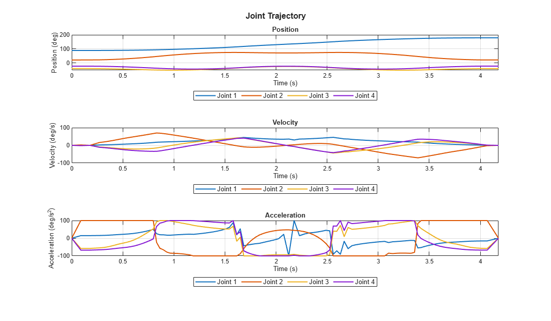
Generate Joint Trajectory

Generate the position, velocity, acceleration, and time vector of the joint trajectory subject to kinematic constraints using the contopptraj function. The function returns a time-optimal trajectory along the path defined by a set of waypoints, constrained by velocity and acceleration limits.

% Define the waypoints to generate trajectory in joint space.
waypoints = jointAngles';

% Define the joint velocity and acceleration constraints on the trajectory.
% Joint velocity and acceleration constraint justification:
%   - Joint acceleration and velocity limits are set based on the joint
%   torque limits, typical values for similar robots, and a safety margin
%   to account for uncertainties and ensure reliable operation.
velLimits = [-180 180; -180 180;-180 180;-180 180]; % deg/s
accelLimits = [-100 100; -100 100;-100 100;-100 100]; % deg/s^2

% Generate the trajectory for each joint of the robot.
[jointPositions,jointVelocities,jointAccelerations,t] = contopptraj(waypoints,velLimits,accelLimits,NumSamples=100);

% Plot the joint trajectory of the robot.
plotJointTrajectory(jointPositions,jointVelocities,jointAccelerations,t);

Generate States

% Create an operating point to define joint position and velocity and
% compute system states.
states = repmat(State,1,length(t)); % Preallocate a vector of state objects

for i = 1:length(t)
    % Create an OperatingPoint to define joint positions and velocities.
    op = simscape.op.OperatingPoint;
    op("Arm_Subsys/Rev_1/Rz/q") = Target(jointPositions(1, i),"deg","High");
    op("Arm_Subsys/Rev_2/Rz/q") = Target(jointPositions(2, i),"deg","High");
    op("Arm_Subsys/Rev_3/Rz/q") = Target(jointPositions(3, i),"deg","High");
    op("Arm_Subsys/Rev_4/Rz/q") = Target(jointPositions(4, i),"deg","High");

    op("Arm_Subsys/Rev_1/Rz/w") = Target(jointVelocities(1, i),"deg/s","High");
    op("Arm_Subsys/Rev_2/Rz/w") = Target(jointVelocities(2, i),"deg/s","High");
    op("Arm_Subsys/Rev_3/Rz/w") = Target(jointVelocities(3, i),"deg/s","High");
    op("Arm_Subsys/Rev_4/Rz/w") = Target(jointVelocities(4, i),"deg/s","High");

    % Compute and store the system state.
    states(i) = computeState(cmb,op);

    % Visualize the manipulator for each iteration
    visualize(cmb,states(i),"robotTrajectory");
end

Perform Dynamics Analysis

Next, determine the maximum lifting force in the -Z direction such that at least one joint reaches its torque limit:

% The motor at each revolute primitive would have a maximum torque capacity.
torqueLimits = [20, 15, 10, 5]; % The torque limit (in N*m) decreases moving from base to tip

% Set up Computed Torque.
actDict = JointActuationDictionary;
compT = RevolutePrimitiveActuationTorque("Computed");
actDict("Arm_Subsys/Rev_1/Rz") = compT;
actDict("Arm_Subsys/Rev_2/Rz") = compT;
actDict("Arm_Subsys/Rev_3/Rz") = compT;
actDict("Arm_Subsys/Rev_4/Rz") = compT;

% Define a handle for the root finder: ratioGuess(f) = maxRatio - 1, where
% ratio is torque/torqueLimit.
% getMaxTorqueRatioForAllStates applies the specified force at the end effector and
% compute the resulting torques for each joint/state, using computeDynamics.
% It returns the maximum absolute torque and the complete torque matrix.
ratioGuess = @(testF) (getMaxTorqueRatioForAllStates(testF, cmb, states, actDict,...
                        jointAccelerations, torqueLimits)) - 1;

% Bracket the guess between lowF and highF, so fzero can locate a root where 
% ratioGuess(f) = 0 (i.e., the joint torque ratio hits 1).
% The function must have opposite signs at these endpoints.
lowF = 0;
highF = 500;

valLow = ratioGuess(lowF);   % if <0 => under limit
valHigh = ratioGuess(highF); % if >0 => over limit

% Solve ratioGuess(f)=0 => means maxRatio=1 => at least one joint is
% exactly at limit.
f_solution = fzero(ratioGuess,[lowF, highF]);

% Retrieve the torque distribution at that force.
[finalRatio, torqueMatrix] = getMaxTorqueRatioForAllStates(f_solution, cmb, states,...
                                                            actDict,jointAccelerations, torqueLimits);

% Now find max force for each orientation, the overall maximum lifting
% capacity will be minimum of all.
maxForces = getMaxForceForEachOrientation(cmb, states, actDict, jointAccelerations, torqueLimits, lowF, highF);

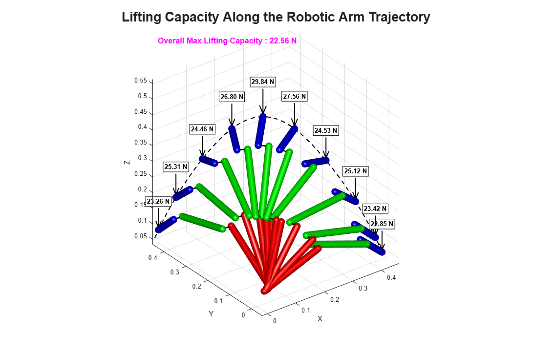
Plot the Results

Retrieve the final poses of each link in 3-D and overlay the manipulator's geometry at key frames along the trajectory, plus the path of the end-effector. We also produce a 2-D plot of the four joint torque history:

trajectory = zeros(numel(states),3);  % Store end-effector positions for plotting

figure('Color','w','Units','pixels','Position',[100 100 1200 800]);
title('Lifting Capacity Along the Robotic Arm Trajectory','FontSize',20);
hold on; grid on;
view(3); axis equal;
xlabel('X'); ylabel('Y'); zlabel('Z');

% Some basic lighting
camlight headlight;
lighting gouraud;
material dull;

% Choose certain key frames to display the arm.
keyFrames = 1:(numel(states)/10):numel(states);
for iter = 1:numel(states)
    % Plot in MATLAB
    link_1_neg = transformation(cmb,"World/W","Arm_Subsys/arm_link_1/NegEnd",states(iter)).Translation.Offset.value;
    link_1_pos = transformation(cmb,"World/W","Arm_Subsys/arm_link_1/PosEnd",states(iter)).Translation.Offset.value;
    link_2_neg = transformation(cmb,"World/W","Arm_Subsys/arm_link_2/NegEnd",states(iter)).Translation.Offset.value;
    link_2_pos = transformation(cmb,"World/W","Arm_Subsys/arm_link_2/PosEnd",states(iter)).Translation.Offset.value;
    link_3_neg = transformation(cmb,"World/W","Arm_Subsys/arm_link_3/NegEnd",states(iter)).Translation.Offset.value;
    link_3_pos = transformation(cmb,"World/W","Arm_Subsys/arm_link_3/PosEnd",states(iter)).Translation.Offset.value;
    
    % Plot only certain frames to reduce clutter
    if (ismember(iter, keyFrames))
        plotRoboticArm(link_1_neg,link_1_pos, ...
                       link_2_neg,link_2_pos, ...
                       link_3_neg,link_3_pos, ...
                       maxForces(iter));

    end

    % Store the end-effector position
    trajectory(iter, :) = link_3_pos';
end

% Highlight the Max Lifting Force on the Plot.
text(0.02, 0.95, 0.02, ...
    sprintf('Overall Max Lifting Capacity : %.2f N',f_solution), ...
    'Units','normalized', ...
    'FontSize',12, ...
    'FontWeight','bold', ...
    'Color','magenta');

% Plot the path of the end-effector.
plot3(trajectory(:, 1),trajectory(:, 2),trajectory(:, 3),'k--','LineWidth',1.5);
hold off;

% Finally, plot the torque profiles for each of the 4 joint primitives.
plotTorques(torqueMatrix,t);

[Joint 1] Max torque = 0.10 Nm 
[Joint 2] Max torque = 15.00 Nm 
[Joint 3] Max torque = 9.37 Nm 
[Joint 4] Max torque = 4.25 Nm 

rmpath(fullfile('DynamicsAnalysisOfARoboticArmInMATLABSupport','Scripts'));