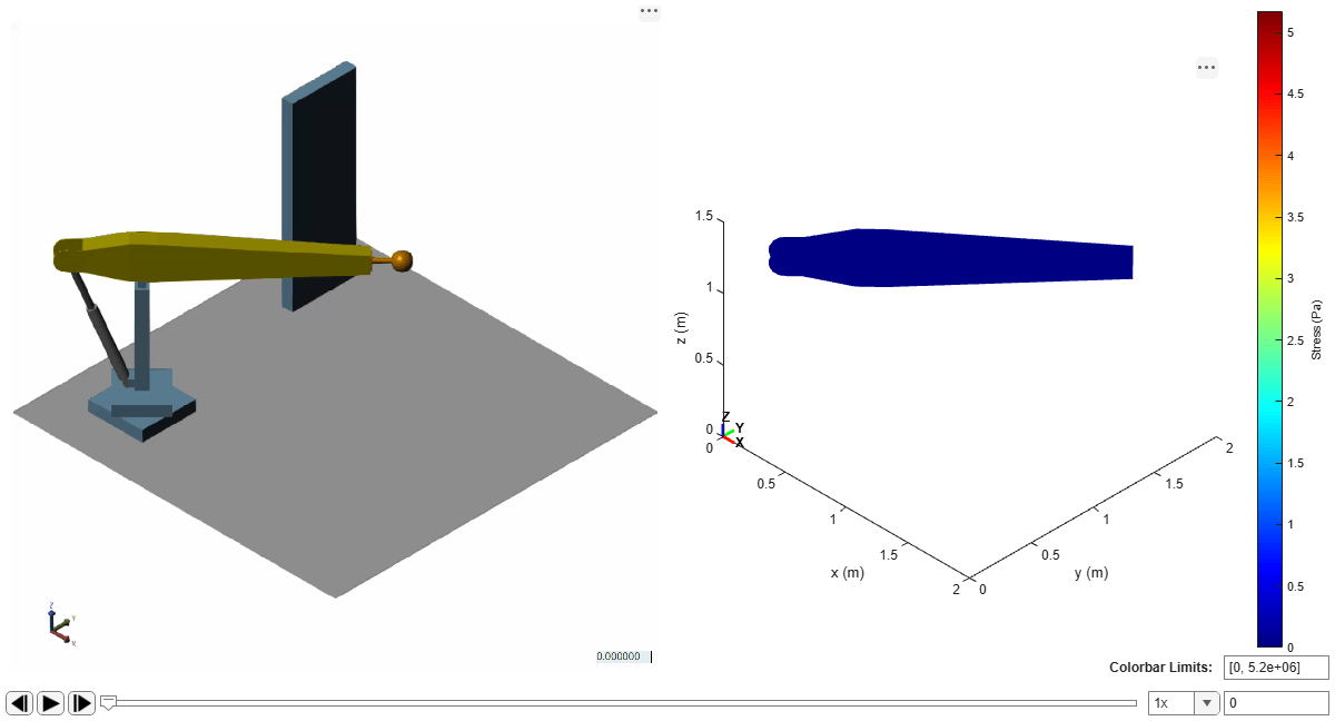
Stress Analysis of an Excavator Dipper Arm

R2026b

This example demonstrates how to perform transient stress analysis of a flexible dipper arm modeled with the Reduced Order Flexible Solid block in Simscape™ Multibody™. During simulation, the Reduced Order Flexible Solid block outputs Reduced Order Flexible Solid and their time derivatives at each time step. These reduced-order degrees of freedom are used to reconstruct the full nodal displacement field and compute stress distribution.

The mapping from reduced-order degrees of freedom to full nodal displacement field is typically provided by the finite-element analysis (FEA) tool used to generate the reduced-order model. In this example, Partial Differential Equation Toolbox™ is used to generate the reduced-order model, reconstruct the nodal displacement field from the reduced-order degrees of freedom, and compute the von Mises stress distribution, while Simscape Multibody is used to perform the multibody simulation of the flexible dipper arm and to log its reduced-order degrees of freedom.

At a high level, the workflow in this example consists of the following steps:

1. Generate a reduced-order model of the dipper arm using Partial Differential Equation Toolbox.

2. Simulate the multibody dynamics of the dipper arm using Reduced Order Flexible Solid block in Simscape Multibody.

3. Log the reduced-order degrees of freedom and their time derivatives to MATLAB®.

4. Reconstruct the nodal displacements and compute von Mises stress from the logged reduced-order degrees of freedom using the evaluateVonMisesStress (Partial Differential Equation Toolbox) and reconstructSolution (Partial Differential Equation Toolbox) methods from Partial Differential Equation Toolbox.

5. Visualize a 3D animation of the flexible dipper-arm motion and associated stress distributions using the pdeplot3D (Partial Differential Equation Toolbox) function and MATLAB graphics in a custom MATLAB app.

Step 1: Generate the Reduced-Order Model

To generate the reduced-order model via Partial Differential Equation Toolbox, we first define the CAD geometry of the dipper arm along with its relevant material properties. We then discretize the geometry into a finite-element mesh and specify the interface frames to define how the dipper arm connects to the rest of the multibody system. Finally, we specify a frequency range within which to retain the fixed interface modes and compute a reduced-order model by using the function reduce (Partial Differential Equation Toolbox). This entire workflow is discussed in more detail in the example Model an Excavator Dipper Arm as a Flexible Body.

In the present example, we use a pre-generated reduced-order model that is loaded from a MAT file and stored in the variable romData. This reduced-order model uses material properties of steel, but the Young's modulus is intentionally scaled down to make the dipper arm more compliant for better illustration of the deformations and stress distributions. The reduced-order model data serves two purposes in this workflow: it provides the necessary data (mass matrix, stiffness matrix, interface frame locations, and visualization data) for the Reduced Order Flexible Solid block (Step 2), and provides the ReducedStructuralModel object for recovering the full nodal solution and stresses after the simulation (Step 4). To regenerate this data for different material properties or mesh settings, you can update and run the script GenerateROM.m.

addpath(genpath("StressAnalysisExcavatorDipperArmSupport"));
romFileName = "DipperArmROMSoftenedSteel.mat";
load(romFileName);

Step 2: Integrate the Reduced-Order Model into the Simscape Multibody Model

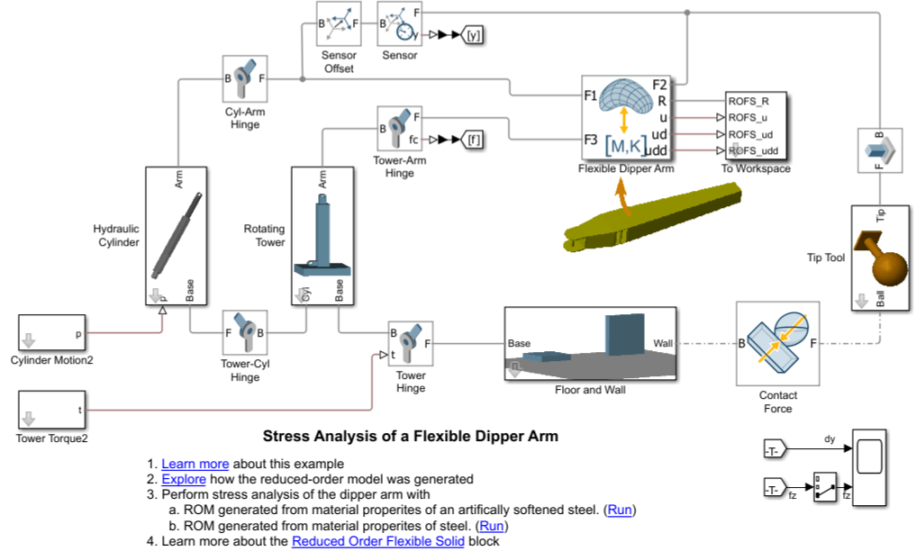
Once the reduced-order model of the dipper arm is generated, it is used to set up the necessary parameters of the Reduced Order Flexible Solid block in Simscape Multibody, as shown in the model ReducedOrderFlexibleSolidStressAnalysis. In this model, the excavator dipper arm is part of a test rig which swings the arm to bring it in contact with a rigid wall. This model is adapted from the example Using the Reduced Order Flexible Solid Block - Flexible Dipper Arm - MATLAB & Simulink.

Step 3: Log the Reduced Order Degrees of Freedom

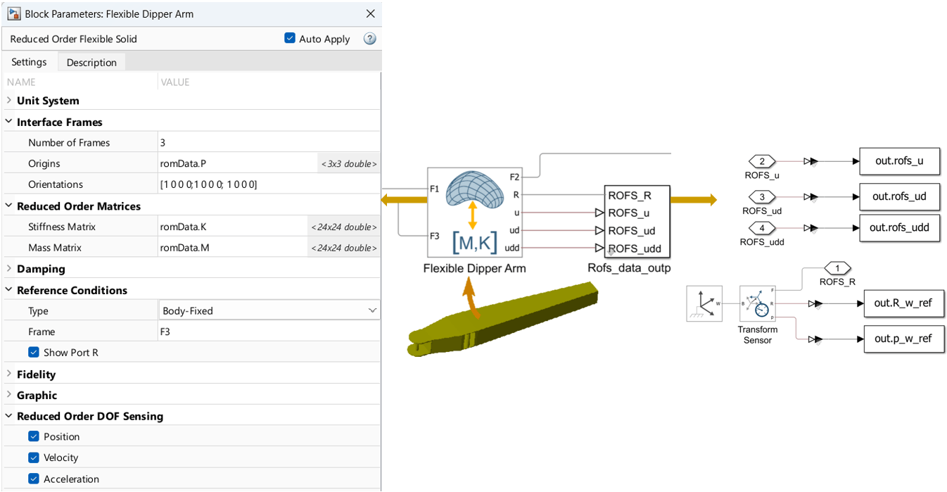
The Reduced Order Flexible Solid block is configured to log the following during model simulation:

• The reduced-order degrees of freedom (position) and their time derivatives (velocity, acceleration) - these capture the deformation of the body with respect to the block's reference frame

• The rotation matrix and position vector between the world frame and the block's reference frame

The reduced-order degrees of freedom and their time derivatives are used in Step 4 for recovering the nodal displacements and the stresses, whereas the transforms between the world frame and the block's reference frame are used in Step 5 to visualize the 3D animation of the deforming body with respect to the world frame.

% Run the simulation and log the reduced-order degrees of freedom to MATLAB
mdlname = "ReducedOrderFlexibleSolidStressAnalysis";
open_system(mdlname);
out = sim(mdlname);

% Extract the reduced‑order degrees of freedom and their time derivatives
% from the logged data.
u = out.rofs_u.Data(:,:);
ud = out.rofs_ud.Data(:,:);
udd = out.rofs_udd.Data(:,:);
timeVec = out.rofs_u.Time;

% Extract the transforms between the World frame and the Reduced Order
% Flexible Solid block's reference frame R from the logged data.
rotm_w_ref = out.rotm_w_ref.Data;
p_w_ref = out.p_w_ref.Data;

Step 4: Reconstruct Full Nodal Solution and Compute von Mises Stress

Once the reduced-order degrees of freedom and their time derivatives are logged to the MATLAB workspace, they are used to recover the nodal displacements and stresses using the following two functions from Partial Differential Equation Toolbox:

• reconstructSolution - recovers the full nodal solution from the reduced-order degrees of freedom for all the logged time steps

• evaluateVonMisesStress - computes von Mises stress at every node in the mesh for all the logged time steps

% Recover full-model transient structural solution
structuralResults = reconstructSolution(romData.rom, u, ud, udd, timeVec);

% Compute the von Mises stress values at the mesh nodes for all the logged
% time steps
vonMisesStressVal = evaluateVonMisesStress(structuralResults);

Step 5: Visualization

To visualize the stress distribution and the deformed shape with respect to the reference frame of the mesh at a single time step, we use the function pdeplot3D. Here we plot the stress distribution at a time step when the dipper arm is in contact with the wall.

% Select a representative time step when the dipper arm is in contact with
% the wall. During contact, the arm bends primarily about the Y-axis of the
% Reduced Order Flexible Solid block's reference frame R. Therefore, we
% find the time step at which the reduced-order degree of freedom
% corresponding to thetaY of interface frame 2 (located at the tip of the
% dipper arm) reaches its largest magnitude.

% Compute the index of the reduced-order degree of freedom corresponding to
% thetaY of interface frame 2.

% The Reduced Order Flexible Solid block outputs the reduced-order degrees
% of freedom with the following ordering per interface frame: [X Y Z thetaX
% thetaY thetaZ]
dofPerFrame = 6;
frameIdx = 2;          % interface frame 2
thetaYLocalIdx = 5;    % [X Y Z thetaX thetaY thetaZ] -> thetaY = 5
thetaYDOFIdxFrame2 = (frameIdx-1)*dofPerFrame + thetaYLocalIdx;

% Get the time step at which the reduced-order degree of freedom
% corresponding to thetaY of interface frame 2 has the largest magnitude
[~, tIdx] = max(abs(u(thetaYDOFIdxFrame2,:)));

% Plot the stress distribution at the selected time step
%
% Note: The red triad displayed by pdeplot3D has the same orientation as
% the Reduced Order Flexible Solid block's reference frame R, but is
% displayed at a different origin.
pdeplot3D(romData.rom.Mesh,...
    ColorMapData=vonMisesStressVal(:,tIdx),...
    Deformation=struct(...
    'ux', structuralResults.Displacement.ux(:,tIdx),...
    'uy', structuralResults.Displacement.uy(:,tIdx),...
    'uz', structuralResults.Displacement.uz(:,tIdx)),...
    DeformationScaleFactor=1)

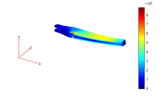
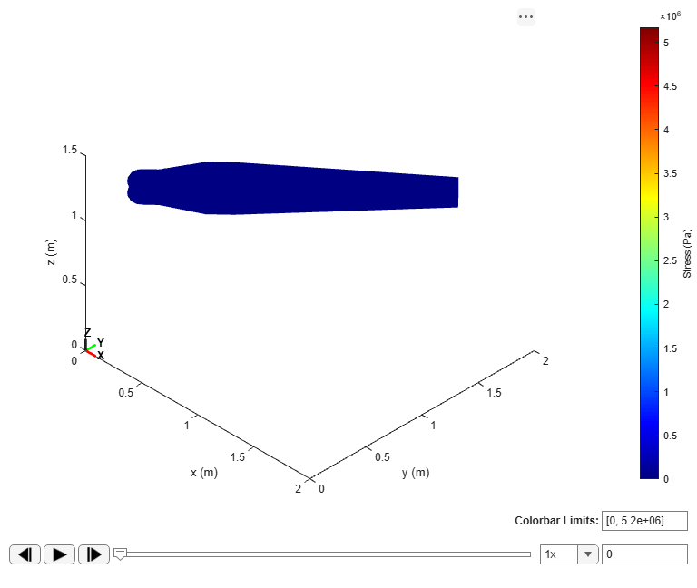
The static plot above shows a single time step. To visualize the full time-history as an animation, we use a custom MATLAB app (StressAnimationApp). It visualizes the 3D animation of the flexible dipper-arm with respect to the world frame and the associated stress distributions using pdeplot3D and MATLAB's handle graphics.

% Set up the parameters needed by StressAnimationApp
mesh = romData.rom.Mesh;

deformationData = struct("ux", structuralResults.Displacement.ux,...
                         "uy", structuralResults.Displacement.uy,...
                         "uz", structuralResults.Displacement.uz,...
                         "rotm_worldToROFSRef", rotm_w_ref,...
                         "pos_worldToROFSRef", p_w_ref);

% In this example, the 3D animation uses color limits that are fixed across
% all time-steps for consistent visualization of the stress distributions.
% The upper limit is chosen as the 98th percentile of the nodal stresses at
% the time step containing the global maximum stress value (instead of using the
% global maximum). We do this because the dipper arm mesh has a few nodes
% with very high localized stresses that would otherwise skew the color
% scale. For the lower limit, we choose the global minimum von Mises Stress
% value.
maxStressesPerTimeStep = max(vonMisesStressVal);
[~, tMaxIndex] = max(maxStressesPerTimeStep);
colorbarLimits = [min(vonMisesStressVal(:)), prctile(vonMisesStressVal(:,tMaxIndex),98)];

% Visualize the von Mises stress and 3D animation of the dipper arm
% simulation.
StressAnimationApp(mesh, deformationData, vonMisesStressVal,...
    timeVec, ColorLimits=colorbarLimits, Title="DipperArmStressAnalysis");

The app can also display the stress animation in sync with the multibody animation of the dipper arm. This view illustrates how the stress distributions on the dipper arm evolve within the broader context of the multibody system.

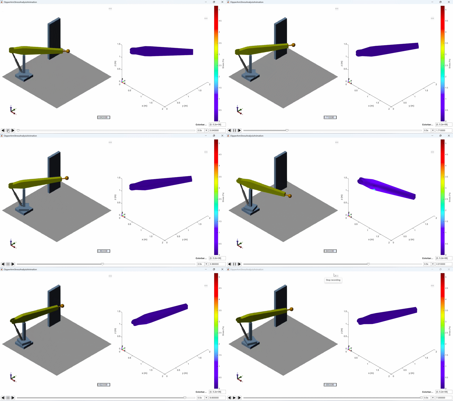
To show this, we pass a pre-generated video of the multibody animation of the dipper arm as an optional argument to the app. For a different simulation configuration, you can regenerate the appropriate multibody animation video via smwritevideo by uncommenting the code below.

% Path to the multibody animation video
videoFile = fullfile('StressAnalysisExcavatorDipperArmSupport','Data', erase(romFileName,'.mat') + "Animation.mp4");

% Uncomment the following lines to regenerate the video of the Multibody animation.
% To ensure that the frames of the multibody animation are in close
% synchronization with the frames of the stress animation, we set the video
% frame rate based on the sample time used to log the reduced-order degrees
% of freedom.

% videoFrameRate = 1/params.rofsOut.ts;
% if isfile(videoFile) 
%     delete(videoFile)
% end
% smwritevideo(mdlname, videoFile, 'FrameRate', videoFrameRate, 'VideoFormat', 'MPEG-4', 'FrameSize', [800 800]);

% Launch the stress animation app with the pre-generated multibody animation video.
StressAnimationApp(mesh, deformationData, vonMisesStressVal, ...
    timeVec, ColorLimits=colorbarLimits, Title="DipperArmStressAnalysisAnimation", ...
    VideoFile=videoFile);