Analysis of Covariance
Introduction to Analysis of Covariance
Analysis of covariance is a technique for analyzing grouped data having a response (y, the variable to be predicted) and a predictor (x, the variable used to do the prediction). Using analysis of covariance, you can model y as a linear function of x, with the coefficients of the line possibly varying from group to group.
Analysis of Covariance Tool
The aoctool function opens
an interactive graphical environment for fitting and prediction with
analysis of covariance (ANOCOVA) models. It fits the following models
for the ith group:
Same mean | y = α + ε |
Separate means | y = (α + αi) + ε |
Same line | y = α + βx + ε |
Parallel lines | y = (α + αi) + βx + ε |
Separate lines | y = (α + αi) + (β + βi)x + ε |
For example, in the parallel lines model the intercept varies from one group to the next, but the slope is the same for each group. In the same mean model, there is a common intercept and no slope. In order to make the group coefficients well determined, the tool imposes the constraints
The following steps describe the use of aoctool.
Load the data. The Statistics and Machine Learning Toolbox™ data set
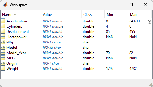
carsmall.matcontains information on cars from the years 1970, 1976, and 1982. This example studies the relationship between the weight of a car and its mileage, and whether this relationship has changed over the years. To start the demonstration, load the data set.load carsmallThe Workspace Browser shows the variables in the data set.
You can also use
aoctoolwith your own data.Start the tool. The following command calls
aoctoolto fit a separate line to the column vectorsWeightandMPGfor each of the three model groups defined inModel_Year. The initial fit models the y variable,MPG, as a linear function of the x variable,Weight.[h,atab,ctab,stats] = aoctool(Weight,MPG,Model_Year);
See the
aoctoolfunction reference page for detailed information about callingaoctool.Examine the output. The graphical output consists of a main window with a plot, a table of coefficient estimates, and an analysis of variance table. In the plot, each
Model_Yeargroup has a separate line. The data points for each group are coded with the same color and symbol, and the fit for each group has the same color as the data points.
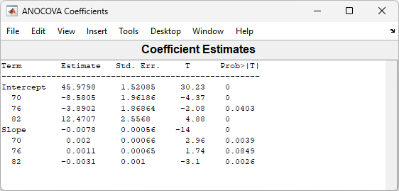
The coefficients of the three lines appear in the figure titled ANOCOVA Coefficients. You can see that the slopes are roughly –0.0078, with a small deviation for each group:
Model year 1970: y = (45.9798 – 8.5805) + (–0.0078 + 0.002)x + ε
Model year 1976: y = (45.9798 – 3.8902) + (–0.0078 + 0.0011)x + ε
Model year 1982: y = (45.9798 + 12.4707) + (–0.0078 – 0.0031)x + ε
Because the three fitted lines have slopes that are roughly similar, you may wonder if they really are the same. The
Model_Year*Weightinteraction expresses the difference in slopes, and the ANOVA table shows a test for the significance of this term. With an F statistic of 5.23 and a p value of 0.0072, the slopes are significantly different.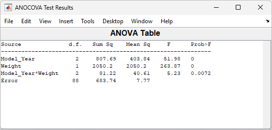
Constrain the slopes to be the same. To examine the fits when the slopes are constrained to be the same, return to the ANOCOVA Prediction Plot window and use the Model pop-up menu to select a
Parallel Linesmodel. The window updates to show the following graph.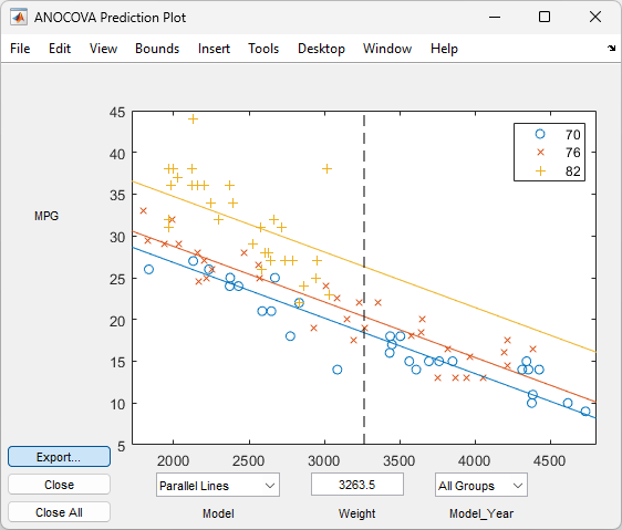
Though this fit looks reasonable, it is significantly worse than the
Separate Linesmodel. Use the Model pop-up menu again to return to the original model.
Confidence Bounds
The example in Analysis of Covariance Tool provides estimates of the relationship
between MPG and Weight for each Model_Year,
but how accurate are these estimates? To find out, you can superimpose
confidence bounds on the fits by examining them one group at a time.
In the Model_Year menu at the lower right of the figure, change the setting from
All Groupsto 82. The data and fits for the other groups are dimmed, and confidence bounds appear around the 82 fit.
The dashed lines form an envelope around the fitted line for model year 82. Under the assumption that the true relationship is linear, these bounds provide a 95% confidence region for the true line. Note that the fits for the other model years are well outside these confidence bounds for
Weightvalues between2000and3000.Sometimes it is more valuable to be able to predict the response value for a new observation, not just estimate the average response value. Use the
aoctoolfunction Bounds menu to change the definition of the confidence bounds fromLinetoObservation. The resulting wider intervals reflect the uncertainty in the parameter estimates as well as the randomness of a new observation.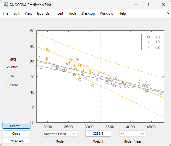
Like the
polytoolfunction, theaoctoolfunction has cross hairs that you can use to manipulate theWeightand watch the estimate and confidence bounds along the y-axis update. These values appear only when a single group is selected, not whenAll Groupsis selected.
Multiple Comparisons
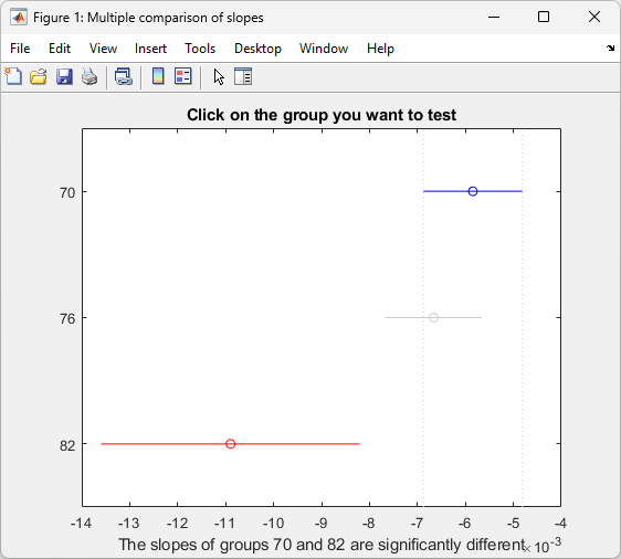
You can perform a multiple comparison test by using the stats output
structure from aoctool as input to the multcompare function. The multcompare function
can test either slopes, intercepts, or population marginal means (the
predicted MPG of the mean weight for each group). The example in Analysis of Covariance Tool shows that
the slopes are not all the same, but could it be that two are the
same and only the other one is different? You can test that hypothesis.
multcompare(stats,0.05,"on","","s")
    1.0000    2.0000   -0.0012    0.0008    0.0029    0.6043
    1.0000    3.0000    0.0013    0.0051    0.0088    0.0049
    2.0000    3.0000    0.0005    0.0042    0.0079    0.0209
This matrix shows that the estimated difference between the intercepts of groups 1 and 2 (1970 and 1976) is 0.0008, and a confidence interval for the difference is [–0.0012, 0.0029]. There is no significant difference between the two. There are significant differences, however, between the intercept for 1982 and each of the other two. The graph shows the same information.
Note that the stats structure was created
in the initial call to the aoctool function, so
it is based on the initial model fit (typically a separate-lines model).
If you change the model interactively and want to base your multiple
comparisons on the new model, you need to run aoctool again
to get another stats structure, this time specifying
your new model as the initial model.