Automated Feature Engineering for Classification
R2026bThe gencfeatures
function enables you to automate the feature engineering process in the context of a machine
learning workflow. Before passing tabular training data to a classifier, you can create new
features from the predictors in the data by using gencfeatures. Use the
returned data to train the classifier.
Generate new features based on your machine learning workflow.
To generate features for an interpretable binary classifier, use the default
TargetLearnervalue of"linear"in the call togencfeatures. You can then use the returned data to train a binary linear classifier. For an example, see Interpret Linear Model with Generated Features.To generate features that can lead to better model accuracy, specify
TargetLearner="bag"orTargetLearner="gaussian-svm"in the call togencfeatures. You can then use the returned data to train a bagged ensemble classifier or a binary support vector machine (SVM) classifier with a Gaussian kernel, respectively. For an example, see Generate New Features to Improve Bagged Ensemble Accuracy.
To better understand the generated features, use the describe function
of the FeatureTransformer
object. To apply the same training set feature transformations to a test or validation set,
use the transform function
of the FeatureTransformer object.
Interpret Linear Model with Generated Features
Use automated feature engineering to generate new features. Train a linear classifier using the generated features. Interpret the relationship between the generated features and the trained model.
Load the patients data set. Create a table from a subset of the variables. Display the first few rows of the table.
load patients
Tbl = table(Age,Diastolic,Gender,Height,SelfAssessedHealthStatus, ...
    Systolic,Weight,Smoker);
head(Tbl)
    Age    Diastolic      Gender      Height    SelfAssessedHealthStatus    Systolic    Weight    Smoker
    ___    _________    __________    ______    ________________________    ________    ______    ______

    38        93        {'Male'  }      71           {'Excellent'}            124        176      true
    43        77        {'Male'  }      69           {'Fair'     }            109        163      false
    38        83        {'Female'}      64           {'Good'     }            125        131      false
    40        75        {'Female'}      67           {'Fair'     }            117        133      false
    49        80        {'Female'}      64           {'Good'     }            122        119      false
    46        70        {'Female'}      68           {'Good'     }            121        142      false
    33        88        {'Female'}      64           {'Good'     }            130        142      true
    40        82        {'Male'  }      68           {'Good'     }            115        180      false
Generate 10 new features from the variables in Tbl. Specify the Smoker variable as the response. By default, gencfeatures assumes that the new features will be used to train a binary linear classifier.
rng("default") % For reproducibility
[T,NewTbl] = gencfeatures(Tbl,"Smoker",10)
T =
  FeatureTransformer with properties:

                     Type: 'classification'
            TargetLearner: 'linear'
    NumEngineeredFeatures: 10
      NumOriginalFeatures: 0
         TotalNumFeatures: 10
NewTbl = 100×11 table
    zsc(Systolic.^2)    eb8(Diastolic)    q8(Systolic)    eb8(Systolic)    q8(Diastolic)    zsc(kmd9)    zsc(sin(Age))    zsc(sin(Weight))    zsc(Height-Systolic)    zsc(kmc1)    Smoker
    ________________    ______________    ____________    _____________    _____________    _________    _____________    ________________    ____________________    _________    ______

         0.15379              8                6                4                8           -1.7207        0.50027            0.19202               0.40418            0.76177    true
         -1.9421              2                1                1                2          -0.22056        -1.1319            -0.4009                2.3431             1.1617    false
         0.30311              4                6                5                5           0.57695        0.50027             -1.037              -0.78898            -1.4456    false
        -0.85785              2                2                2                2           0.83391         1.1495             1.3039               0.85162          -0.010294    false
        -0.14125              3                5                4                4             1.779        -1.3083           -0.42387              -0.34154            0.99368    false
        -0.28697              1                4                3                1           0.67326         1.3761           -0.72529               0.40418             1.3755    false
          1.0677              6                8                6                6          -0.42521         1.5181           -0.72529               -1.5347            -1.4456    true
         -1.1361              4                2                2                5          -0.79995         1.1495            -1.0225                1.2991             1.1617    false
         -1.1361              3                2                2                3          -0.80136        0.46343             1.0806                1.2991             -1.208    false
        -0.71693              5                3                3                6           0.37961       -0.51304            0.16741               0.55333            -1.4456    false
         -1.2734              2                1                1                2            1.2572         1.3025             1.0978                1.4482          -0.010294    false
         -1.1361              1                2                2                1             1.001        -1.2545            -1.2194                1.0008          -0.010294    false
         0.60534              1                6                5                1          -0.98493       -0.11998             -1.211             -0.043252             -1.208    false
          1.0677              8                8                6                8          -0.27307         1.4659             1.2168              -0.34154            0.24706    true
         -1.2734              3                1                1                4           0.93395        -1.3633           -0.17603                1.0008          -0.010294    false
          1.0677              7                8                6                8          -0.91396          -1.04            -1.2109              -0.49069            0.24706    true
      ⋮
T is a FeatureTransformer object that can be used to transform new data, and newTbl contains the new features generated from the Tbl data.
To better understand the generated features, use the describe object function of the FeatureTransformer object. For example, inspect the first two generated features.
describe(T,1:2)
                           Type        IsOriginal    InputVariables                            Transformations
                        ___________    __________    ______________    _______________________________________________________________

    zsc(Systolic.^2)    Numeric          false         Systolic        power(  ,2)
                                                                       Standardization with z-score (mean = 15119.54, std = 1667.5858)
    eb8(Diastolic)      Categorical      false         Diastolic       Equal-width binning (number of bins = 8)
The first feature in newTbl is a numeric variable, created by first squaring the values of the Systolic variable and then converting the results to z-scores. The second feature in newTbl is a categorical variable, created by binning the values of the Diastolic variable into 8 bins of equal width.
Use the generated features to fit a linear classifier without any regularization.
Mdl = fitclinear(NewTbl,"Smoker",Lambda=0);Plot the coefficients of the predictors used to train Mdl. Note that fitclinear expands categorical predictors before fitting a model.
p = length(Mdl.Beta);
[sortedCoefs,expandedIndex] = sort(Mdl.Beta,ComparisonMethod="abs");
sortedExpandedPreds = Mdl.ExpandedPredictorNames(expandedIndex);
bar(sortedCoefs,Horizontal="on")
yticks(1:2:p)
yticklabels(sortedExpandedPreds(1:2:end))
xlabel("Coefficient")
ylabel("Expanded Predictors")
title("Coefficients for Expanded Predictors")
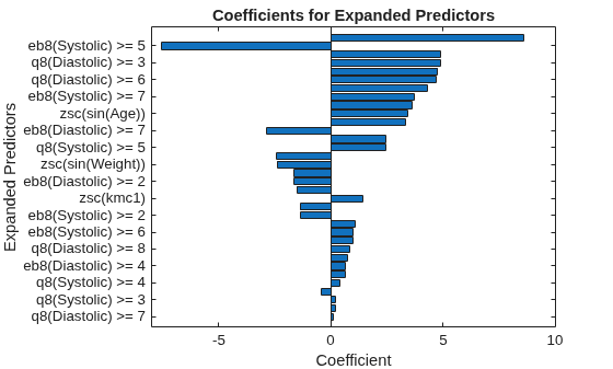
Identify the predictors whose coefficients have larger absolute values.
bigCoefs = abs(sortedCoefs) >= 4;
flip(sortedExpandedPreds(bigCoefs))
ans = 1×7 cell
    {'zsc(Systolic.^2)'}    {'eb8(Systolic) >= 5'}    {'eb8(Diastolic) >= 3'}    {'q8(Diastolic) >= 3'}    {'q8(Systolic) >= 6'}    {'q8(Diastolic) >= 6'}    {'zsc(Height-Systolic)'}
You can use partial dependence plots to analyze the categorical features whose levels have large coefficients in terms of absolute value. For example, inspect the partial dependence plot for the q8(Diastolic) variable, whose levels q8(Diastolic) >= 3 and q8(Diastolic) >= 6 have coefficients with large absolute values. These two levels correspond to noticeable changes in the predicted scores.
plotPartialDependence(Mdl,"q8(Diastolic)",Mdl.ClassNames,NewTbl);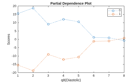
Generate New Features to Improve Bagged Ensemble Accuracy
Use gencfeatures to engineer new features before training a bagged ensemble classifier. To avoid data leakage, partition the data into two sets and generate the feature transformations on one of the data sets. Then, apply the same feature transformations to the remaining data set. Observe the 5-fold cross-validation performance of a bagged ensemble trained using progressively more features, including the original and engineered features.
Read the sample file CreditRating_Historical.dat into a table. The predictor data consists of financial ratios and industry sector information for a list of corporate customers. The response variable consists of credit ratings assigned by a rating agency. Preview the first few rows of the data set.
creditrating = readtable("CreditRating_Historical.dat");
head(creditrating)
ID WC_TA RE_TA EBIT_TA MVE_BVTD S_TA Industry Rating
_____ ______ ______ _______ ________ _____ ________ _______
62394 0.013 0.104 0.036 0.447 0.142 3 {'BB' }
48608 0.232 0.335 0.062 1.969 0.281 8 {'A' }
42444 0.311 0.367 0.074 1.935 0.366 1 {'A' }
48631 0.194 0.263 0.062 1.017 0.228 4 {'BBB'}
43768 0.121 0.413 0.057 3.647 0.466 12 {'AAA'}
39255 -0.117 -0.799 0.01 0.179 0.082 4 {'CCC'}
62236 0.087 0.158 0.049 0.816 0.324 2 {'BBB'}
39354 0.005 0.181 0.034 2.597 0.388 7 {'AA' }
Because each value in the ID variable is a unique customer ID, that is, length(unique(creditrating.ID)) is equal to the number of observations in creditrating, the ID variable is a poor predictor. Remove the ID variable from the table, and convert the Industry variable to a categorical variable.
creditrating = removevars(creditrating,"ID");
creditrating.Industry = categorical(creditrating.Industry);
Convert the Rating response variable to a categorical variable.
creditrating.Rating = categorical(creditrating.Rating, ...
    ["AAA","AA","A","BBB","BB","B","CCC"]);
Partition the data into a feature engineering set and an evaluation set. Use approximately 30% of the observations to learn the feature transformations, and use the remaining 70% of the observations to perform 5-fold cross-validation. Cross-validation provides a less noisy estimate of model performance than holdout validation.
rng("default") % For reproducibility of the partition
c = cvpartition(creditrating.Rating,Holdout=0.70);
feIndices = training(c);
evalIndices = test(c);
creditFE = creditrating(feIndices,:);
creditEval = creditrating(evalIndices,:);
Use the feature engineering data to generate new features to fit a bagged ensemble. By default, the gencfeatures function includes any original features that can be used as predictors by a bagged ensemble. Request a total of 12 features, namely the 6 original features in creditFE and up to 6 engineered features.
T = gencfeatures(creditFE,"Rating",12,TargetLearner="bag")
T =
  FeatureTransformer with properties:

                     Type: 'classification'
            TargetLearner: 'bag'
    NumEngineeredFeatures: 6
      NumOriginalFeatures: 6
         TotalNumFeatures: 12
Create newCreditEval by applying the transformations stored in the object T to the evaluation data.
newCreditEval = transform(T,creditEval)
newCreditEval = 2752×13 table
    WC_TA     RE_TA     EBIT_TA    MVE_BVTD    S_TA     Industry    WC_TA+MVE_BVTD    RE_TA+MVE_BVTD    EBIT_TA.*MVE_BVTD    RE_TA.*MVE_BVTD    MVE_BVTD./S_TA    RE_TA.*S_TA    Rating
    ______    ______    _______    ________    _____    ________    ______________    ______________    _________________    _______________    ______________    ___________    ______

     0.013     0.104     0.036      0.447      0.142       3             0.46             0.551             0.016092             0.046488           3.1479          0.014768      BB
     0.232     0.335     0.062      1.969      0.281       8            2.201             2.304              0.12208              0.65962           7.0071          0.094135      A
     0.311     0.367     0.074      1.935      0.366       1            2.246             2.302              0.14319              0.71015           5.2869           0.13432      A
     0.194     0.263     0.062      1.017      0.228       4            1.211              1.28             0.063054              0.26747           4.4605          0.059964      BBB
     0.121     0.413     0.057      3.647      0.466       12           3.768              4.06              0.20788               1.5062           7.8262           0.19246      AAA
    -0.117    -0.799      0.01      0.179      0.082       4            0.062             -0.62              0.00179             -0.14302           2.1829         -0.065518      CCC
     0.087     0.158     0.049      0.816      0.324       2            0.903             0.974             0.039984              0.12893           2.5185          0.051192      BBB
      0.11     0.337     0.045      3.835      0.812       4            3.945             4.172              0.17257               1.2924           4.7229           0.27364      AAA
    -0.108    -0.615     0.017      0.145      0.104       11           0.037             -0.47             0.002465            -0.089175           1.3942          -0.06396      CCC
     0.008     0.121      0.03      2.109      0.446       9            2.117              2.23              0.06327              0.25519           4.7287          0.053966      A
     0.031     0.045     0.039      0.816      0.301       6            0.847             0.861             0.031824              0.03672            2.711          0.013545      BB
    -0.015     0.178     0.021      3.087      0.685       9            3.072             3.265             0.064827              0.54949           4.5066           0.12193      A
    -0.097    -0.004     0.024      0.673      0.178       1            0.576             0.669             0.016152            -0.002692           3.7809         -0.000712      BB
     0.262     0.429     0.064      2.355      0.292       5            2.617             2.784              0.15072               1.0103           8.0651           0.12527      AA
     0.251     0.283     0.063       0.94       0.28       5            1.191             1.223              0.05922              0.26602           3.3571           0.07924      BBB
     0.048     0.247     0.042      2.941      0.493       8            2.989             3.188              0.12352              0.72643           5.9655           0.12177      AA
      ⋮
The first six columns of newCreditEval correspond to the original features, the next six columns correspond to the engineered features, and the last column corresponds to the response variable.
Compute the 5-fold cross-validation accuracy of a bagged ensemble trained on progressively more features. That is, first evaluate the performance of the model trained using only the WC_TA original feature. Then, evaluate the performance of the model trained using the WC_TA and RE_TA original features. Continue until you evaluate the performance of the model trained on all 12 features (original and engineered).
cvAccuracy = nan(12,1);
rating = newCreditEval.Rating;
for k = 1:12
    cvMdl = fitcensemble(newCreditEval(:,1:k),rating, ...
        Method="Bag",KFold=5);
    cvAccuracy(k) = 1 - kfoldLoss(cvMdl);
end

results = table((1:12)',cvAccuracy, ...
    VariableNames=["NumFeatures","5-FoldAccuracy"])
results = 12×2 table
    NumFeatures    5-FoldAccuracy
    ___________    ______________

         1            0.26635
         2            0.50836
         3            0.54142
         4             0.7311
         5            0.74201
         6            0.75436
         7            0.76199
         8            0.76781
         9            0.76381
        10            0.76054
        11            0.75654
        12            0.76163
Visualize the accuracy as the number of features increases.
bar(cvAccuracy)
xlabel("Number of Predictors Used")
ylabel("5-Fold Cross-Validation Accuracy")
title("Bagged Ensemble Performance")
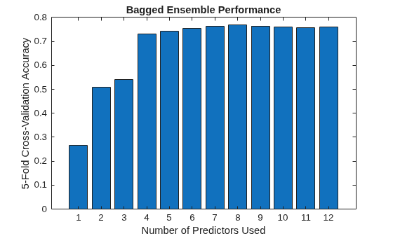
The plot shows that adding a small number of engineered features (for a total of around 8 features) slightly improves the 5-fold cross-validation accuracy of the bagged ensemble. However, adding further engineered features does not improve the model performance and can even degrade performance. This behavior is expected in practice. The first few engineered features tend to capture strong nonlinear interactions or informative transformations that are not well represented in the original feature space. Once these dominant patterns are captured, additional engineered features are often weakly informative or redundant with existing predictors. As the number of predictors increases, the bagged ensemble fits a higher-dimensional feature space, which increases the model variance and makes the classifier more sensitive to noise in the training data. Even though bagging reduces variance relative to a single tree, the process does not eliminate overfitting when many low-signal features are included. This example shows the motivation for applying feature engineering conservatively: adding a small number of well-chosen engineered features can improve predictive performance, but indiscriminately adding many features can introduce noise and reduce generalization accuracy.
See Also
gencfeatures | FeatureTransformer | describe | transform | fitclinear | fitcensemble | fitcsvm | plotPartialDependence | genrfeatures

