geostat

Geometric mean and variance

Syntax

[m,v] = geostat(p)

Description

[m,v] = geostat(p) returns the mean m and variance v of a geometric distribution with the corresponding probability parameter in p. For more information, see Geometric Distribution Mean and Variance.

Examples

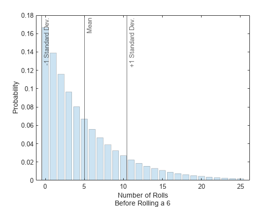
Visualize Mean and Standard Deviation of Geometric Distribution

Roll a fair die repeatedly until you successfully get a 6. The associated geometric distribution models the number of times you roll the die before the result is a 6. Determine the mean and variance of the distribution, and visualize the results.

Because the die is fair, the probability of successfully rolling a 6 in any given trial is p = 1/6. Compute the mean and variance of the geometric distribution.

p = 1/6;
[m,v] = geostat(p)

m = 
5.0000

v = 
30.0000

Notice that the mean m is $$(1-p)/p$$ and the variance v is $$(1-p)/p^2$$.

m2 = (1-p)/p

m2 = 
5.0000

v2 = (1-p)/p^2

v2 = 
30.0000

Evaluate the probability density function (pdf), or probability mass function (pmf), at the points x = 0,1,2,...,25.

rng("default") % For reproducibility
x = 0:25;
y = geopdf(x,p);

Plot the pdf values. Indicate the mean, one standard deviation below the mean, and one standard deviation above the mean.

bar(x,y,"FaceAlpha",0.2,"EdgeAlpha",0.2);
xline([m-sqrt(v) m m+sqrt(v)],"-", ...
    ["-1 Standard Dev.","Mean","+1 Standard Dev."])
xlabel(["Number of Rolls","Before Rolling a 6"])
ylabel("Probability")

Compute Mean and Variance of Multiple Geometric Distributions

Create a probability vector that contains three different parameter values.

• The first parameter corresponds to a geometric distribution that models the number of times you toss a coin before the result is heads.

• The second parameter corresponds to a geometric distribution that models the number of times you roll a four-sided die before the result is a 4.

• The third parameter corresponds to a geometric distribution that models the number of times you roll a six-sided die before the result is a 6.

p = [1/2 1/4 1/6];

Compute the mean and variance of each geometric distribution.

[m,v] = geostat(p)

m = 1×3

    1.0000    3.0000    5.0000

v = 1×3

    2.0000   12.0000   30.0000

The returned values indicate that, for example, the mean of a geometric distribution with probability parameter p = 1/4 is 3, and the variance of the distribution is 12.

Input Arguments

p — Probability of success

scalar in the range [0,1] | array of scalars in the range [0,1]

Probability of success in a single trial, specified as a scalar or an array of scalars in the range [0,1]. To compute the means and variances of multiple distributions, specify the distribution parameters p using an array of scalar values.

Example: 0.5

Example: [1/2 1/3]

Data Types: single | double

Output Arguments

m — Mean

numeric scalar | array of numeric scalars

Mean of the geometric distribution, returned as a numeric scalar or an array of numeric scalars. m is the same size as p, and each element in m is the mean of the geometric distribution specified by the corresponding element in p.

v — Variance

numeric scalar | array of numeric scalars

Variance of the geometric distribution, returned as a numeric scalar or an array of numeric scalars. v is the same size as p, and each element in v is the variance of the geometric distribution specified by the corresponding element in p.

More About

Geometric Distribution Mean and Variance

The geometric distribution is a one-parameter family of curves that models the number of failures before a success occurs in a series of independent trials. Each trial results in either success or failure, and the probability of success in any individual trial is constant. For example, if you toss a coin, the geometric distribution models the number of tails observed before the result is heads. The geometric distribution is discrete, existing only on the nonnegative integers.

The mean of the geometric distribution is $$\text{mean}=\frac{1-p}{p},$$ and the variance of the geometric distribution is $$\mathrm{var}=\frac{1-p}{p^2},$$ where p is the probability of success.

References

[1] Abramowitz, M., and I. A. Stegun. Handbook of Mathematical Functions. New York: Dover, 1964.

[2] Evans, M., N. Hastings, and B. Peacock. Statistical Distributions. 2nd ed., Hoboken, NJ: John Wiley & Sons, Inc., 1993.

Extended Capabilities

C/C++ Code Generation
Generate C and C++ code using MATLAB® Coder™.

GPU Arrays

Accelerate code by running on a graphics processing unit (GPU) using Parallel Computing Toolbox™.

This function fully supports GPU arrays. For more information, see Run MATLAB Functions on a GPU (Parallel Computing Toolbox).

Version History

Introduced before R2006a