incrementalTrainingOptions

R2026b

Options for training incremental neural network

Since R2026b

Syntax

options = incrementalTrainingOptions(solverName)

options = incrementalTrainingOptions(solverName,Name=Value)

Description

options = incrementalTrainingOptions(solverName) returns incremental training options for the specified solver. Use the incremental training options object when you create an incrementalClassificationNeuralNetwork or incrementalRegressionNeuralNetwork model object.

options = incrementalTrainingOptions(solverName,Name=Value) specifies options using one or more name-value arguments. For example, incrementalTrainingOptions("freerex",L2Regularization=1e-5) specifies to train with the FreeRex solver and an L2 regularization strength of 1e–5.

Examples

Create Incremental Training Options Object

Create a training options object that contains the default FreeRex solver options for an incremental neural network learning object.

FreeRexOptions=incrementalTrainingOptions("freerex")

FreeRexOptions = 
  TrainingOptionsFREEREX

         UpdateMethod: "coordinate-wise"
    RegularizerFactor: 2.2361
     L2Regularization: 1.0000e-05


  Properties, Methods

FreeRexOptions is a TrainingOptionsFREEREX object. Create an incremental neural network classification model with a maximum of five expected classes using the default FreeRex solver options.

IncrementalMdl = incrementalClassificationNeuralNetwork(MaxNumClasses=5,TrainingOptions=FreeRexOptions)

IncrementalMdl = 
  incrementalClassificationNeuralNetwork

                   IsWarm: 0
                  Metrics: [1×2 table]
               ClassNames: [1×0 double]
           ScoreTransform: 'none'
               LayerSizes: 10
              Activations: "relu"
    OutputLayerActivation: "softmax"
                   Solver: "freerex"


  Properties, Methods

IncrementalMdl is an incrementalClassificationNeuralNetwork model object. The solver options are stored in the object's TrainingOptions property.

Create Incremental Learner with Little Prior Information

When you create a neural network classification model for incremental learning, you can specify the maximum number of classes that you expect the model to process (MaxNumClasses name-value argument). As you fit the model to incoming batches of data by using an incremental fitting function, the model collects new classes in its ClassNames property. If the specified maximum number of classes is inaccurate, one of the following occurs:

• Before an incremental fitting function processes the expected maximum number of classes, the model is not warm. Consequently, the updateMetrics and updateMetricsAndFit functions do not measure performance metrics.

• If the number of classes exceeds the maximum expected, the incremental fitting function issues an error.

This example shows how to create a neural network classification model for incremental learning when the only information you specify is the expected maximum number of classes in the data. Also, the example illustrates the consequences when incremental fitting functions process all expected classes early and late in the sample.

For this example, consider training a device to predict whether a subject is sitting, standing, walking, running, or dancing based on biometric data measured on the subject. Therefore, the device has a maximum of five classes from which to choose.

Process Expected Maximum Number of Classes Early in Sample

Create an incremental neural network model for multiclass learning. Specify a maximum of five classes in the data, and standardize the predictor values.

MdlEarly = incrementalClassificationNeuralNetwork(MaxNumClasses=5)

MdlEarly = 
  incrementalClassificationNeuralNetwork

                   IsWarm: 0
                  Metrics: [1×2 table]
               ClassNames: [1×0 double]
           ScoreTransform: 'none'
               LayerSizes: 10
              Activations: "relu"
    OutputLayerActivation: "softmax"
                   Solver: "minibatch-lbfgs"


  Properties, Methods

MdlEarly is an incrementalClassificationNeuralNetwork model object. MdlEarly must be fit to data before you can use it to perform any other operations.

Display the default training period values associated with the model object.

MdlEarly.TrainingOptions.TuningPeriod

ans = 
1000

MdlEarly.MetricsWarmupPeriod

ans = 
1000

When you use fit and updateMetricsAndFit to fit the model, these functions:

• Use the first incoming 1000 observations to tune the initial learning rate for the solver

• Process the next 1000 observations during the warm-up period

Once the model has been fit to all expected classes and at least 2000 observations, the model is warm, and the fit and updateMetricsAndFit functions compute and store performance metrics.

Load the human activity data set. Randomly shuffle the data.

load humanactivity
n = numel(actid);
rng(1); % For reproducibility
idx = randsample(n,n);
X = feat(idx,:);
Y = actid(idx);

For details on the data set, enter Description at the command line.

Fit the incremental model to the training data by using the updateMetricsAndFit function. Simulate a data stream by processing chunks of 50 observations at a time. At each iteration:

• Process 50 observations.

• Overwrite the previous incremental model with a new one fitted to the incoming observations.

• Store the cumulative metrics and the window metrics to see how they evolve during incremental learning.

% Preallocation
numObsPerChunk = 50;
nchunk = floor(n/numObsPerChunk);
mc = array2table(zeros(nchunk,2),VariableNames=["Cumulative" "Window"]);
IsWarm = zeros(nchunk+1,1);    
% Incremental learning
for j = 1:nchunk
    ibegin = min(n,numObsPerChunk*(j-1) + 1);
    iend = min(n,numObsPerChunk*j);
    idx = ibegin:iend;    
    MdlEarly = updateMetricsAndFit(MdlEarly,X(idx,:),Y(idx));
    mc{j,:} = MdlEarly.Metrics{"MinimalCost",:};
    IsWarm(j + 1) = MdlEarly.IsWarm;
end

MdlEarly is an incrementalClassificationNeuralNetwork model object trained on all the data in the stream. During incremental learning and after the model is warm, updateMetricsAndFit checks the performance of the model on the incoming observations, and then fits the model to those observations.

To see how the IsWarm property and performance metrics evolve during training, plot them on separate tiles.

t = tiledlayout(2,1);
nexttile
plot(IsWarm)
ylabel("IsWarm")
xlim([0 nchunk])
ylim([0 1.1])
xline((MdlEarly.TrainingOptions.TuningPeriod + ...
    MdlEarly.MetricsWarmupPeriod)/numObsPerChunk,"r-.")
nexttile
h = plot(mc.Variables);
xlim([0 nchunk])
ylabel("Minimal Cost")
xline((MdlEarly.TrainingOptions.TuningPeriod + ...
    MdlEarly.MetricsWarmupPeriod)/numObsPerChunk,"r-.")
legend(h,mc.Properties.VariableNames)
xlabel(t,"Iteration")

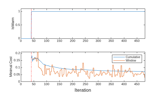
The plots indicate that updateMetricsAndFit performs the following actions:

• Compute the performance metrics after the tuning and metrics warm-up periods (red vertical line) only.

• Compute the cumulative metrics during each iteration.

• Compute the window metrics after processing 200 observations (4 iterations).

Process Expected Maximum Number of Classes Late in Sample

Create a different neural network model for incremental learning for the objective.

MdlLate = incrementalClassificationNeuralNetwork(MaxNumClasses=5, ...
    Standardize=true)

MdlLate = 
  incrementalClassificationNeuralNetwork

                   IsWarm: 0
                  Metrics: [1×2 table]
               ClassNames: [1×0 double]
           ScoreTransform: 'none'
               LayerSizes: 10
              Activations: "relu"
    OutputLayerActivation: "softmax"
                   Solver: "minibatch-lbfgs"


  Properties, Methods

Move all observations labeled with class 5 to the end of the sample.

idx5 = Y == 5;
Xnew = [X(~idx5,:); X(idx5,:)];
Ynew = [Y(~idx5) ;Y(idx5)];

Fit the incremental model and plot the results.

mcnew = array2table(zeros(nchunk,2),VariableNames=["Cumulative" "Window"]);

for j = 1:nchunk
    ibegin = min(n,numObsPerChunk*(j-1) + 1);
    iend   = min(n,numObsPerChunk*j);
    idx = ibegin:iend;    
    MdlLate = updateMetricsAndFit(MdlLate,Xnew(idx,:),Ynew(idx));
    mcnew{j,:} = MdlLate.Metrics{"MinimalCost",:};
 end

figure
h = plot(mcnew.Variables);
xlim([0 nchunk]);
ylabel("Minimal Cost")
xline((MdlLate.TrainingOptions.TuningPeriod + ...
    MdlLate.MetricsWarmupPeriod)/numObsPerChunk,"r-.")
xline(sum(~idx5)/numObsPerChunk,"g-.")
legend(h,mcnew.Properties.VariableNames,Location="best")
xlabel("Iteration")

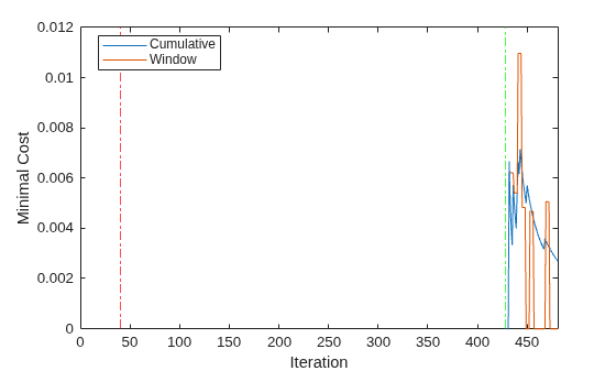
The updateMetricsAndFit function trains the model throughout incremental learning, but the function starts tracking performance metrics only after the model is fit to all expected number of classes (the green vertical line).

Input Arguments

solverName — Solver for training neural network

"minibatch-lbfgs" | "freerex"

Solver for training incremental neural network, specified as one of these values:

Value	Solver Name	More Information
"minibatch-lbfgs"	Mini-Batch Limited-memory Broyden–Fletcher–Goldfarb–Shanno (LBFGS)	Limited-Memory BFGS
"freerex"	FreeRex	FreeRex

Name-Value Arguments

Specify optional pairs of arguments as Name1=Value1,...,NameN=ValueN, where Name is the argument name and Value is the corresponding value. Name-value arguments must appear after other arguments, but the order of the pairs does not matter.

Example: options = incrementalTrainingOptions("freerex",UpdateMethod="l2-norm")

Mini-batch LBFGS and FreeRex Options

L2Regularization — L2 regularization term strength

1e-5 (default) | nonnegative scalar

L2 regularization term strength, specified as a nonnegative scalar. Larger values apply stronger regularization to the model coefficients. This argument applies when solverName is "minibatch-lbfgs" or "freerex".

Data Types: double | single

Mini-batch LBFGS Options

BatchSize — Mini-batch size

10 (default) | positive integer

Mini-batch size, specified as a positive integer. At each iteration, the software estimates the subgradient using BatchSize observations from the training data.

Example: BatchSize=100

Data Types: single | double

GradientTolerance — Relative convergence tolerance

1e-6 (default) | nonnegative scalar

Relative convergence tolerance on the L-infinity norm of the gradient, specified as one of these values:

• Positive scalar — Stop training when the relative gradient is less than or equal to the specified value.

• 0 — Do not stop training based on the relative gradient.

Let $${ℒ}_t$$ be the loss function at training iteration t, $$\nabla {ℒ}_t$$ be the gradient of the loss function with respect to the weights and biases at iteration t, and $$\nabla {ℒ}_0$$ be the gradient of the loss function at an initial point. If $$\max \left|\nabla {ℒ}_t\right|\le a\cdot \text{GradientTolerance}$$, where $$a=\max \left(1,\min \left|{ℒ}_t\right|,\max \left|\nabla {ℒ}_0\right|\right)$$, then the training process terminates.

Example: GradientTolerance=1e-5

Data Types: single | double

HistorySize — Number of state updates to store

10 (default) | positive integer

Number of state updates to store, specified as a positive integer. Values between 3 and 20 suit most tasks. Larger values use more memory but can improve convergence. The LBFGS algorithm uses a history of gradient calculations to approximate the Hessian matrix recursively. For more information, see Limited-Memory BFGS.

Example: GradientTolerance=5

Data Types: single | double

InitialInverseHessianFactor — Scaling factor for initial inverse Hessian approximation

1 (default) | positive scalar

Initial value that characterizes the approximate inverse Hessian matrix, specified as a positive scalar.

To save memory, the LBFGS algorithm does not store and invert the dense Hessian matrix B. Instead, the algorithm uses the approximation $$B_{k-m}^{-1}\approx {\lambda }_{k}I$$, where m is the history size, the inverse Hessian factor $${\lambda }_k$$ is a scalar, and I is the identity matrix. The algorithm then stores the scalar inverse Hessian factor only. The algorithm updates the inverse Hessian factor at each step.

The initial inverse hessian factor is the value of $${\lambda }_0$$.

For more information, see Limited-Memory BFGS.

Example: InitialInverseHessianFactor=1.5

Data Types: single | double

InitialLearnRate — Initial learning rate

"auto" (default) | positive scalar or "auto"

Initial learning rate, specified as a positive scalar or "auto". When set to "auto", the solver determines the initial learning rate during a tuning period controlled by TuningPeriod and TuningSubsetSize. When set to a numeric value, the tuning period is disabled (TuningPeriod and TuningSubsetSize are set to 0).

If the learning rate is too low, then training can take many iterations to converge. If the learning rate is too high, then training might converge to a suboptimal result or diverge.

Example: InitialLearnRater=1.5

Data Types: double | single | string

InitialStepSize — Approximate maximum absolute value of the first optimization step

[] (default) | "auto" | positive scalar

Initial step size, specified as one of these values:

• [] — Do not use an initial step size to determine the initial Hessian approximation.

• "auto" — Determine the initial step size automatically. The software uses an initial step size of $$\Vert s_0{\Vert }_{\infty }=\frac{1}{2}\Vert W_0{\Vert }_{\infty }+0.1$$, where W₀ are the initial learnable parameters of the network.

• Positive real scalar — Use the specified value as the initial step size $$\Vert s_0{\Vert }_{\infty }$$.

Example: InitialStepSize=2

Data Types: single | double

LearnRateSchedule — Learning rate schedule

"decaying" (default) | "constant"

Learning rate schedule, specified as "decaying" or "constant". A decaying schedule reduces the learning rate over time, while a constant schedule keeps it fixed at the initial value.

Example: LearnRateSchedule="constant"

Data Types: string | char

LineSearchMethod — Method to find suitable learning rate

"weak-wolfe" (default) | "strong-wolfe" | "backtracking"

Method to find suitable learning rate, specified as one of these values:

• "weak-wolfe" — Search for a learning rate that satisfies the weak Wolfe conditions. This method maintains a positive definite approximation of the inverse Hessian matrix.

• "strong-wolfe" — Search for a learning rate that satisfies the strong Wolfe conditions. This method maintains a positive definite approximation of the inverse Hessian matrix.

• "backtracking" — Search for a learning rate that satisfies sufficient decrease conditions. This method does not maintain a positive definite approximation of the inverse Hessian matrix.

Example: LineSearchMethod="backtracking"

Data Types: string | char

MaxNumIterations — Maximum number of LBFGS iterations per mini-batch

10 (default) | positive integer

Maximum number of iterations per mini-batch LBFGS step, specified as a positive integer

Example: MaxNumIterations=50

Data Types: single | double

MaxNumLineSearchIterations — Maximum number of line search iterations

20 (default) | positive integer

Maximum number of line search iterations to determine the learning rate, specified as a positive integer.

Example: MaxNumLineSearchIterations=50

Data Types: single | double

StepTolerance — L2 norm step size tolerance

1e-5 (default) | nonnegative scalar | 0

L2 norm step size tolerance, specified as a nonnegative scalar.

If the step size at some iteration is smaller than StepTolerance, then the training process terminates.

Example: StepTolerance=1e-4

Data Types: single | double

TuningPeriod — Number of observations for learning rate tuning

1000 (default) | nonnegative integer

Number of observations for learning rate tuning, specified as a nonnegative integer scalar. The solver uses the first TuningSubsetSize observations for testing, and the next TuningPeriod-TuningSubsetSize observations to determine a good initial learning rate when InitialLearnRate is "auto". If you specify TuningPeriod without specifying TuningSubsetSize, then TuningSubsetSize is set to ceil(0.1*TuningPeriod).

Example: TuningPeriod=500

Data Types: single | double

TuningSubsetSize — Number of observations in each tuning subset

100 (default) | nonnegative integer

Number of observations in each tuning subset, specified as a nonnegative integer scalar. The value must be less than or equal to TuningPeriod. If you specify TuningSubsetSize without specifying TuningPeriod, then TuningPeriod is set to 10*TuningSubsetSize.

Example: TuningSubsetSize=50

Data Types: single | double

FreeRex Options

RegularizerFactor — Regularizer scaling factor

sqrt(5) (default) | positive scalar

Regularizer scaling factor, specified as a positive scalar. This factor scales the regularization term in the FreeRex algorithm.

Example: RegularizerFactor=2

Data Types: double | single

UpdateMethod — Parameter update method

"coordinate-wise" (default) | "l2-norm"

Parameter update method, specified as one of the following:

• "coordinate-wise" — Apply updates independently for each weight.

• "l2-norm" — Apply updates based on the L2-norm of the gradient.

Example: UpdateMethod="l2-norm"

Data Types: string | char

Output Arguments

options — Training options object for incremental neural network model

TrainingOptionsMiniBatchLBFGS object | TrainingOptionsFREEREX object

Training options object for incremental neural network model, returned as a TrainingOptionsMiniBatchLBFGS or TrainingOptionsFREEREX object depending on the specified solverName. Use this object with the TrainingOptions name-value argument of the incremental neural network learning functions to control solver behavior.

Algorithms

Limited-Memory BFGS

The LBFGS algorithm [4] is a quasi-Newton method that approximates the Broyden-Fletcher-Goldfarb-Shanno (BFGS) algorithm. Use the LBFGS algorithm for small networks and data sets that you can process in a single batch.

The algorithm updates learnable parameters W at iteration k+1 using the update step given by

$$W_{k+1}=W_k-{\eta }_k{B}_k^{-1}\nabla J(W_k),$$

where W_k denotes the weights at iteration k, $${\eta }_k$$ is the learning rate at iteration k, B_k is an approximation of the Hessian matrix at iteration k, and $$\nabla J(W_k)$$ denotes the gradients of the loss with respect to the learnable parameters at iteration k.

The LBFGS algorithm computes the matrix-vector product $$B_k^{-1}\nabla J(W_k)$$ directly. The algorithm does not require computing the inverse of B_k.

To compute the matrix-vector product $$B_k^{-1}\nabla J(W_k)$$ directly, the LBFGS algorithm uses this recursive algorithm:

1. Set $$r=B_{k-m}^{-1}\nabla J(W_k)$$, where m is the history size.

2. For $$i=m,\dots ,1$$:

   1. Let $$\beta =\frac{1}{s_{k-i}^{\top }{y}_{k-i}}{y}_{k-i}^{\top }r$$, where $$s_{k-i}$$ and $$y_{k-i}$$ are the step and gradient differences for iteration $$k-i$$, respectively.

   2. Set $$r=r+\text{}{s}_{k-i}\text{}\left(a_{k-i}-\beta \right)$$, where $$a$$ is derived from $$s$$, $$y$$, and the gradients of the loss with respect to the loss function. For more information, see [4].

3. Return $$B_k^{-1}\nabla J(W_k)=r$$.

FreeRex

The FreeRex (Free Regret via Exponential Updates) algorithm [3] is a parameter-free first-order optimizer that automatically adjusts its update magnitudes based on accumulated gradient information. Because there is no learning rate parameter, there is no solver tuning period when you train an incremental learning model object using the FreeRex solver.

L₂ Regularization

Adding a regularization term for the weights to the loss function $$E\left(\theta \right)$$ is one way to reduce overfitting [1], [5]. The regularization term is also called weight decay. The loss function with the regularization term takes the form

$$E_R\left(\theta \right)=E\left(\theta \right)+\lambda \Omega \left(w\right),$$

where $$w$$ is the weight vector, $$\lambda$$ is the regularization factor (coefficient), and the regularization function $$\Omega \left(w\right)$$ is

$$\Omega \left(w\right)=\frac{1}{2}{w}^{T}w.$$

Note that the biases are not regularized [5]. You can specify the regularization factor $$\lambda$$ by using the L2Regularization training option.

References

[1] Bishop, C. M. Pattern Recognition and Machine Learning. Springer, New York, NY, 2006.

[2] Cutkosky, Ashok, and Kwabena Boahen. "Online Convex Optimization with Unconstrained Domains and Losses." NIPS pp. 748-756, 2016.

[3] Cutkosky, Ashok, and Kwabena Boahen. "Online learning without prior information." In Conference on learning theory, pp. 643-677. PMLR, 2017.

[4] Liu, Dong C., and Jorge Nocedal. "On the limited memory BFGS method for large scale optimization." Mathematical programming 45, no. 1 (August 1989): 503-528. https://doi.org/10.1007/BF01589116.

[5] Murphy, K. P. Machine Learning: A Probabilistic Perspective. The MIT Press, Cambridge, Massachusetts, 2012.

[6] Nocedal, J. and S. J. Wright. Numerical Optimization, 2nd ed., New York: Springer, 2006.

Version History

Introduced in R2026b