Build a Map from Lidar Data Using SLAM
This example shows how to process 3-D lidar data from a sensor mounted on a vehicle to progressively build a map and estimate the trajectory of a vehicle using simultaneous localization and mapping (SLAM). In addition to 3-D lidar data, an inertial navigation sensor (INS) is also used to help build the map. Maps built this way can facilitate path planning for vehicle navigation or can be used for localization.
Overview
The Build a Map from Lidar Data example uses 3-D lidar data and IMU readings to progressively build a map of the environment traversed by a vehicle. While this approach builds a locally consistent map, it is suitable only for mapping small areas. Over longer sequences, the drift accumulates into a significant error. To overcome this limitation, this example recognizes previously visited places and tries to correct for the accumulated drift using the graph SLAM approach.
Load and Explore Recorded Data
The data used in this example is part of the Velodyne SLAM Dataset, and represents close to 6 minutes of recorded data. Download the data to a temporary directory.
Note: This download can take a few minutes.
baseDownloadURL = 'https://www.mrt.kit.edu/z/publ/download/velodyneslam/data/scenario1.zip';
dataFolder = fullfile(tempdir,'kit_velodyneslam_data_scenario1',filesep);
options = weboptions('Timeout',Inf);

zipFileName  = dataFolder + "scenario1.zip";

% Get the full file path to the PNG files in the scenario1 folder
pointCloudFilePattern = fullfile(dataFolder,'scenario1','scan*.png');
numExpectedFiles = 2513;

folderExists = exist(dataFolder,'dir');
if ~folderExists
    % Create a folder in a temporary directory to save the downloaded zip
    % file
    mkdir(dataFolder);

    disp('Downloading scenario1.zip (153 MB) ...')
    websave(zipFileName,baseDownloadURL,options);

    % Unzip downloaded file
    unzip(zipFileName,dataFolder);

elseif folderExists && numel(dir(pointCloudFilePattern)) < numExpectedFiles
    % Redownload the data if it got reduced in the temporary directory
    disp('Downloading scenario1.zip (153 MB) ...')
    websave(zipFileName,baseDownloadURL,options);

    % Unzip downloaded file
    unzip(zipFileName,dataFolder)
end
Downloading scenario1.zip (153 MB) ...
Use the helperReadDataset function to read data from the created folder in the form of a timetable. The point clouds captured by the lidar are stored in the form of PNG image files. Extract the list of point cloud file names in the pointCloudTable variable. To read the point cloud data from the image file, use the helperReadPointCloudFromFile function. This function takes an image file name and returns a pointCloud object. The INS readings are read directly from a configuration file and stored in the insDataTable variable.
datasetTable = helperReadDataset(dataFolder,pointCloudFilePattern);

pointCloudTable = datasetTable(:,1);
insDataTable = datasetTable(:,2:end);
Read the first point cloud and display it at the MATLAB® command prompt.
ptCloud = helperReadPointCloudFromFile(pointCloudTable.PointCloudFileName{1});
disp(ptCloud)
pointCloud with properties:
Location: [64×870×3 single]
Count: 55680
XLimits: [-78.4980 77.7062]
YLimits: [-76.8795 74.7502]
ZLimits: [-2.4839 2.6836]
Color: []
Normal: []
Intensity: []
Display the first INS reading. The timetable holds Heading, Pitch, Roll, X, Y, and Z information from the INS.
disp(insDataTable(1,:))
         Timestamps         Heading     Pitch        Roll          X          Y         Z
    ____________________    _______    ________    _________    _______    _______    ______

    13-Jun-2010 06:27:31    1.9154     0.007438    -0.019888    -2889.1    -2183.9    116.47
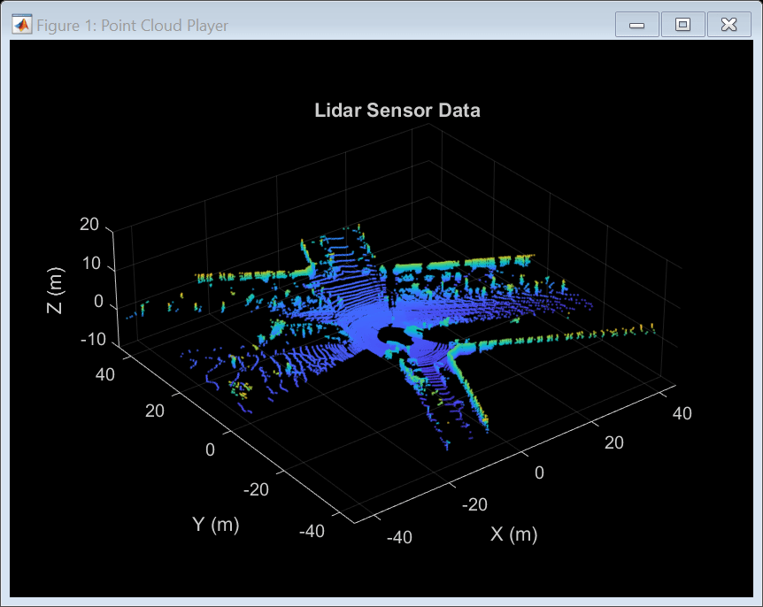
Visualize the point clouds using pcplayer, a streaming point cloud display. The vehicle traverses a path consisting of two loops. In the first loop, the vehicle makes a series of turns and returns to the starting point. In the second loop, the vehicle makes a series of turns along another route and again returns to the starting point.
% Specify limits of the player
xlimits = [-45 45]; % meters
ylimits = [-45 45];
zlimits = [-10 20];

% Create a streaming point cloud display object
lidarPlayer = pcplayer(xlimits,ylimits,zlimits);

% Customize player axes labels
xlabel(lidarPlayer.Axes,'X (m)')
ylabel(lidarPlayer.Axes,'Y (m)')
zlabel(lidarPlayer.Axes,'Z (m)')

title(lidarPlayer.Axes,'Lidar Sensor Data')

% Skip evey other frame since this is a long sequence
skipFrames = 2;
numFrames = height(pointCloudTable);
for n = 1:skipFrames:numFrames

    % Read a point cloud
    fileName = pointCloudTable.PointCloudFileName{n};
    ptCloud = helperReadPointCloudFromFile(fileName);

    % Visualize point cloud
    view(lidarPlayer,ptCloud);

    pause(0.01)
end

Build a Map Using Odometry
First, use the approach explained in the Build a Map from Lidar Data example to build a map. The approach consists of the following steps:
Align Lidar scans: Align successive lidar scans using a point cloud registration technique. This example uses
pcregisterndtfor registering scans. By successively composing these transformations, each point cloud is transformed back to the reference frame of the first point cloud.Combine aligned scans: Generate a map by combining all the transformed point clouds.
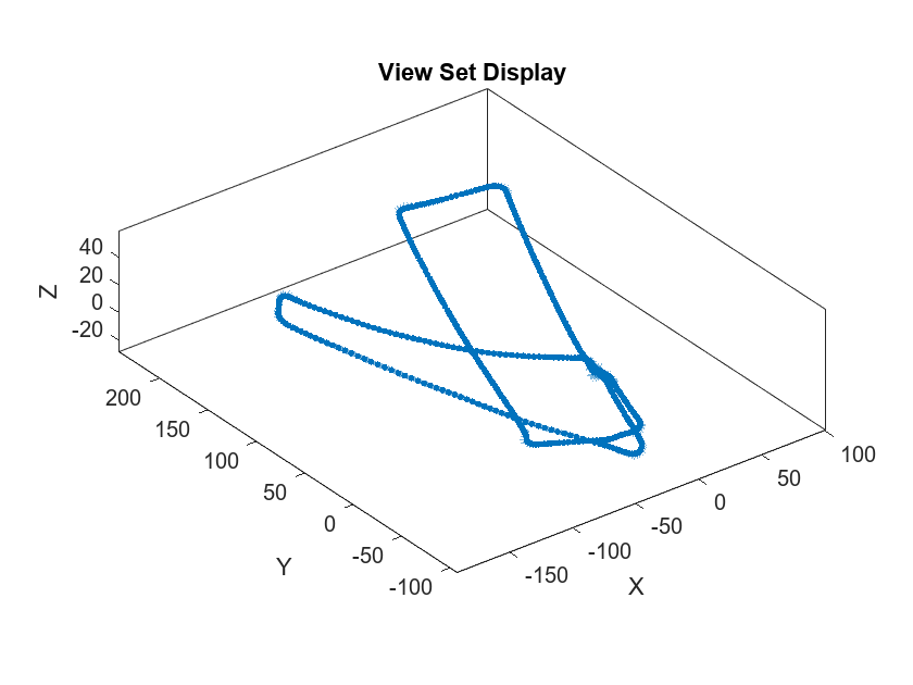
This approach of incrementally building a map and estimating the trajectory of the vehicle is called odometry.
Use a pcviewset object to store and manage data across multiple views. A view set consists of a set of connected views.
Each view stores information associated with a single view. This information includes the absolute pose of the view, the point cloud sensor data captured at that view, and a unique identifier for the view. Add views to the view set using
addView.To establish a connection between views use
addConnection. A connection stores information like the relative transformation between the connecting views, the uncertainty involved in computing this measurement (represented as an information matrix) and the associated view identifiers.Use the
plotmethod to visualize the connections established by the view set. These connections can be used to visualize the path traversed by the vehicle.
hide(lidarPlayer)

% Set random seed to ensure reproducibility
rng(0);

% Create an empty view set
vSet = pcviewset;

% Initialize point cloud processing parameters
downsamplePercent = 0.1;
regGridSize = 3;

% Initialize transformations
absTform = rigidtform3d;  % Absolute transformation to reference frame
relTform = rigidtform3d;  % Relative transformation between successive scans

viewId = 1;
skipFrames = 5;
numFrames = height(pointCloudTable);
displayRate = 100;  % Update display every 100 frames
for n = 1:skipFrames:numFrames

    % Read point cloud
    fileName = pointCloudTable.PointCloudFileName{n};
    ptCloudOrig = helperReadPointCloudFromFile(fileName);

    % Process point cloud
    %   - Segment and remove ground plane
    %   - Segment and remove ego vehicle
    ptCloud = helperProcessPointCloud(ptCloudOrig);

    % Downsample the processed point cloud
    ptCloud = pcdownsample(ptCloud,"random",downsamplePercent);

    firstFrame = (n==1);
    if firstFrame
        % Add first point cloud scan as a view to the view set
        vSet = addView(vSet,viewId,absTform,"PointCloud",ptCloudOrig);

        viewId = viewId + 1;
        ptCloudPrev = ptCloud;
        continue;
    end

    % Use INS to estimate an initial transformation for registration
    initTform = helperComputeInitialEstimateFromINS(relTform, ...
        insDataTable(n-skipFrames:n,:));

    % Compute rigid transformation that registers current point cloud with
    % previous point cloud
    relTform = pcregisterndt(ptCloud,ptCloudPrev,regGridSize, ...
        "InitialTransform",initTform);

    % Update absolute transformation to reference frame (first point cloud)
    absTform = rigidtform3d(absTform.A * relTform.A);

    % Add current point cloud scan as a view to the view set
    vSet = addView(vSet,viewId,absTform,"PointCloud",ptCloudOrig);

    % Add a connection from the previous view to the current view, representing
    % the relative transformation between them
    vSet = addConnection(vSet,viewId-1,viewId,relTform);

    viewId = viewId + 1;

    if mod(viewId,displayRate) == 0
        plot(vSet)
        drawnow
    end

    ptCloudPrev = ptCloud;
    initTform = relTform;
end

title('View Set Display')

The view set object vSet, now holds views and connections. In the Views table of vSet, the AbsolutePose variable specifies the absolute pose of each view with respect to the first view. In the Connections table of vSet, the RelativePose variable specifies relative constraints between the connected views, the InformationMatrix variable specifies, for each edge, the uncertainty associated with a connection.
% Display the first few views and connections
head(vSet.Views)
ViewId AbsolutePose PointCloud
______ ________________ ______________
1 1×1 rigidtform3d 1×1 pointCloud
2 1×1 rigidtform3d 1×1 pointCloud
3 1×1 rigidtform3d 1×1 pointCloud
4 1×1 rigidtform3d 1×1 pointCloud
5 1×1 rigidtform3d 1×1 pointCloud
6 1×1 rigidtform3d 1×1 pointCloud
7 1×1 rigidtform3d 1×1 pointCloud
8 1×1 rigidtform3d 1×1 pointCloud
head(vSet.Connections)
    ViewId1    ViewId2      RelativePose      InformationMatrix
    _______    _______    ________________    _________________

       1          2       1×1 rigidtform3d      {6×6 double}
       2          3       1×1 rigidtform3d      {6×6 double}
       3          4       1×1 rigidtform3d      {6×6 double}
       4          5       1×1 rigidtform3d      {6×6 double}
       5          6       1×1 rigidtform3d      {6×6 double}
       6          7       1×1 rigidtform3d      {6×6 double}
       7          8       1×1 rigidtform3d      {6×6 double}
       8          9       1×1 rigidtform3d      {6×6 double}
Now, build a point cloud map using the created view set. Align the view absolute poses with the point clouds in the view set using pcalign. Specify a grid size to control the resolution of the map. The map is returned as a pointCloud object.
ptClouds = vSet.Views.PointCloud;
absPoses = vSet.Views.AbsolutePose;
mapGridSize = 0.2;
ptCloudMap = pcalign(ptClouds,absPoses,mapGridSize);
Notice that the path traversed using this approach drifts over time. While the path along the first loop back to the starting point seems reasonable, the second loop drifts significantly from the starting point. The accumulated drift results in the second loop terminating several meters away from the starting point.
A map built using odometry alone is inaccurate. Display the built point cloud map with the traversed path. Notice that the map and traversed path for the second loop are not consistent with the first loop.
figure
pcshow(ptCloudMap);
hold on
plot(vSet)
title('Point Cloud Map','Color','w')

Correct Drift Using Pose Graph Optimization
Graph SLAM is a widely used technique for resolving the drift in odometry. The graph SLAM approach incrementally creates a graph, where nodes correspond to vehicle poses and edges represent sensor measurements constraining the connected poses. Such a graph is called a pose graph. The pose graph contains edges that encode contradictory information, due to noise or inaccuracies in measurement. The nodes in the constructed graph are then optimized to find the set of vehicle poses that optimally explain the measurements. This technique is called pose graph optimization.
To create a pose graph from a view set, you can use the createPoseGraph function. This function creates a node for each view, and an edge for each connection in the view set. To optimize the pose graph, you can use the optimizePoseGraph (Navigation Toolbox) function.
A key aspect contributing to the effectiveness of graph SLAM in correcting drift is the accurate detection of loops, that is, places that have been previously visited. This is called loop closure detection or place recognition. Adding edges to the pose graph corresponding to loop closures provides a contradictory measurement for the connected node poses, which can be resolved during pose graph optimization.
Loop closures can be detected using descriptors that characterize the local environment visible to the Lidar sensor. The Scan Context descriptor [1] is one such descriptor that can be computed from a point cloud using the scanContextDescriptor function. This example uses a scanContextLoopDetector object to manage the scan context descriptors that correspond to each view. It uses the detectLoop object function to detect loop closures with a two phase descriptor search algorithm. In the first phase, it computes the ring key subdescriptors to find potential loop candidates. In the second phase, it classifies views as loop closures by thresholding the scan context distance.
% Set random seed to ensure reproducibility
rng(0);

% Create an empty view set
vSet = pcviewset;

% Create a loop closure detector
loopDetector = scanContextLoopDetector;

% Initialize transformations
absTform = rigidtform3d;  % Absolute transformation to reference frame
relTform = rigidtform3d;  % Relative transformation between successive scans

maxTolerableRMSE = 3;  % Maximum allowed RMSE for a loop closure candidate to be accepted

viewId = 1;
for n = 1:skipFrames:numFrames

    % Read point cloud
    fileName = pointCloudTable.PointCloudFileName{n};
    ptCloudOrig = helperReadPointCloudFromFile(fileName);

    % Process point cloud
    %   - Segment and remove ground plane
    %   - Segment and remove ego vehicle
    ptCloud = helperProcessPointCloud(ptCloudOrig);

    % Downsample the processed point cloud
    ptCloud = pcdownsample(ptCloud,"random",downsamplePercent);

    firstFrame = (n==1);
    if firstFrame
        % Add first point cloud scan as a view to the view set
        vSet = addView(vSet,viewId,absTform,"PointCloud",ptCloudOrig);

        % Extract the scan context descriptor from the first point cloud
        descriptor = scanContextDescriptor(ptCloudOrig);

        % Add the first descriptor to the loop closure detector
        addDescriptor(loopDetector,viewId,descriptor)

        viewId = viewId + 1;
        ptCloudPrev = ptCloud;
        continue;
    end

    % Use INS to estimate an initial transformation for registration
    initTform = helperComputeInitialEstimateFromINS(relTform, ...
        insDataTable(n-skipFrames:n,:));

    % Compute rigid transformation that registers current point cloud with
    % previous point cloud
    relTform = pcregisterndt(ptCloud,ptCloudPrev,regGridSize, ...
        "InitialTransform",initTform);

    % Update absolute transformation to reference frame (first point cloud)
    absTform = rigidtform3d(absTform.A * relTform.A);

    % Add current point cloud scan as a view to the view set
    vSet = addView(vSet,viewId,absTform,"PointCloud",ptCloudOrig);

    % Add a connection from the previous view to the current view representing
    % the relative transformation between them
    vSet = addConnection(vSet,viewId-1,viewId,relTform);

    % Extract the scan context descriptor from the point cloud
    descriptor = scanContextDescriptor(ptCloudOrig);

    % Add the descriptor to the loop closure detector
    addDescriptor(loopDetector,viewId,descriptor)

    % Detect loop closure candidates
    loopViewId = detectLoop(loopDetector);

    % A loop candidate was found
    if ~isempty(loopViewId)
        loopViewId = loopViewId(1);

        % Retrieve point cloud from view set
        loopView = findView(vSet,loopViewId);
        ptCloudOrig = loopView.PointCloud;

        % Process point cloud
        ptCloudOld = helperProcessPointCloud(ptCloudOrig);

        % Downsample point cloud
        ptCloudOld = pcdownsample(ptCloudOld,"random",downsamplePercent);

        % Use registration to estimate the relative pose
        [relTform,~,rmse] = pcregisterndt(ptCloud,ptCloudOld, ...
            regGridSize,"MaxIterations",50);

        acceptLoopClosure = rmse <= maxTolerableRMSE;
        if acceptLoopClosure
            % For simplicity, use a constant, small information matrix for
            % loop closure edges
            infoMat = 0.01 * eye(6);

            % Add a connection corresponding to a loop closure
            vSet = addConnection(vSet,loopViewId,viewId,relTform,infoMat);
        end
    end

    viewId = viewId + 1;

    ptCloudPrev = ptCloud;
    initTform = relTform;
end
Create a pose graph from the view set by using the createPoseGraph method. The pose graph is a digraph object with:
Nodes containing the absolute pose of each view
Edges containing the relative pose constraints of each connection
G = createPoseGraph(vSet);
disp(G)
  digraph with properties:

    Edges: [539×3 table]
    Nodes: [503×2 table]
% Display view set to display loop closure detections
figure
hG = plot(vSet);

% Update axes limits to focus on loop closure detections
xlim([-50 50]);
ylim([-100 50]);

% Find and highlight loop closure connections
loopEdgeIds = find(abs(diff(G.Edges.EndNodes,1,2)) > 1);
highlight(hG,'Edges',loopEdgeIds,'EdgeColor','red','LineWidth',3)
title('Loop Closure Connections')

Optimize the pose graph using optimizePoseGraph (Navigation Toolbox).
optimG = optimizePoseGraph(G,'g2o-levenberg-marquardt');

vSetOptim = updateView(vSet,optimG.Nodes);
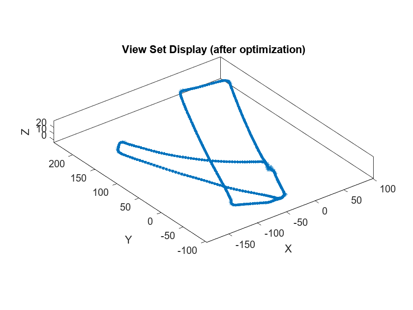
Display the view set with optimized poses. Notice that the detected loops are now merged, resulting in a more accurate trajectory.
figure
plot(vSetOptim)
title('View Set Display (after optimization)')
The absolute poses in the optimized view set can now be used to build a more accurate map. Use the pcalign function to align the view set point clouds with the optimized view set absolute poses into a single point cloud map. Specify a grid size to control the resolution of the created point cloud map.
mapGridSize = 0.2;
ptClouds = vSetOptim.Views.PointCloud;
absPoses = vSetOptim.Views.AbsolutePose;
ptCloudMap = pcalign(ptClouds,absPoses,mapGridSize);

figure
pcshow(ptCloudMap);

% Overlay view set display
hold on
plot(vSetOptim);
title('Point Cloud Map (after optimization)','Color','w')

While accuracy can still be improved, this point cloud map is significantly more accurate.
Speed Up SLAM Workflow Using GPU Code Generation
Most functionality in this example supports GPU code generation. For an example that shows how to do 3-D Lidar SLAM on an NVIDIA® GPU, refer to the following example:
3-D Lidar SLAM Using Other Registration Algorithms
This example uses pcregisterndt to align successive point clouds. You can refer to the following examples that provide an alternate approach to registering point clouds:
Build a Map with Lidar Odometry and Mapping (LOAM) Using Unreal Engine Simulation (Lidar Toolbox): uses
pcregisterloam(Lidar Toolbox) to register the point clouds andpcmaploam(Lidar Toolbox) to refine the alignment.Design Lidar SLAM Algorithm Using Unreal Engine Simulation Environment: uses
pcregistericpto register the point clouds andscanContextLoopDetectorto detect loop closures.Aerial Lidar SLAM Using FPFH Descriptors (Lidar Toolbox): uses a feature detection and matching approach to find the relative pose between point clouds and
pcregistericpto refine the alignment.
References
G. Kim and A. Kim, "Scan Context: Egocentric Spatial Descriptor for Place Recognition Within 3D Point Cloud Map," 2018 IEEE/RSJ International Conference on Intelligent Robots and Systems (IROS), Madrid, 2018, pp. 4802-4809.
Supporting Functions and Classes
helperReadDataset reads data from specified folder into a timetable.
function datasetTable = helperReadDataset(dataFolder,pointCloudFilePattern)
%helperReadDataset Read Velodyne SLAM Dataset data into a timetable
%   datasetTable = helperReadDataset(dataFolder) reads data from the
%   folder specified in dataFolder into a timetable. The function
%   expects data from the Velodyne SLAM Dataset.
%
%   See also fileDatastore, helperReadINSConfigFile.

% Create a file datastore to read in files in the right order
fileDS = fileDatastore(pointCloudFilePattern,'ReadFcn', ...
    @helperReadPointCloudFromFile);

% Extract the file list from the datastore
pointCloudFiles = fileDS.Files;

imuConfigFile = fullfile(dataFolder,'scenario1','imu.cfg');
insDataTable = helperReadINSConfigFile(imuConfigFile);

% Delete the bad row from the INS config file
insDataTable(1447,:) = [];

% Remove columns that will not be used
datasetTable = removevars(insDataTable, ...
    {'Num_Satellites','Latitude','Longitude','Altitude','Omega_Heading', ...
     'Omega_Pitch','Omega_Roll','V_X','V_Y','V_ZDown'});

datasetTable = addvars(datasetTable,pointCloudFiles,'Before',1, ...
    'NewVariableNames',"PointCloudFileName");
end
helperProcessPointCloud processes a point cloud by removing points belonging to the ground plane and the ego vehicle.
function ptCloud = helperProcessPointCloud(ptCloudIn,method)
%helperProcessPointCloud Process pointCloud to remove ground and ego vehicle
%   ptCloud = helperProcessPointCloud(ptCloudIn,method) processes
%   ptCloudIn by removing the ground plane and the ego vehicle.
%   method can be "planefit" or "rangefloodfill".
%
%   See also pcfitplane, pointCloud/findPointsInCylinder.

arguments
    ptCloudIn (1,1) pointCloud
    method          string      {mustBeMember(method,["planefit","rangefloodfill"])} = "rangefloodfill"
end

isOrganized = ~ismatrix(ptCloudIn.Location);

if (method=="rangefloodfill" && isOrganized)
    % Segment ground using floodfill on range image
    groundFixedIdx = segmentGroundFromLidarData(ptCloudIn, ...
        "ElevationAngleDelta",11);
else
    % Segment ground as the dominant plane with reference normal
    % vector pointing in positive z-direction
    maxDistance = 0.4;
    maxAngularDistance = 5;
    referenceVector= [0 0 1];

    [~,groundFixedIdx] = pcfitplane(ptCloudIn,maxDistance, ...
        referenceVector,maxAngularDistance);
end

if isOrganized
    groundFixed = false(size(ptCloudIn.Location,1),size(ptCloudIn.Location,2));
else
    groundFixed = false(ptCloudIn.Count,1);
end
groundFixed(groundFixedIdx) = true;

% Segment ego vehicle as points within a cylindrical region of the sensor
sensorLocation = [0 0 0];
egoRadius = 3.5;
egoFixed = findPointsInCylinder(ptCloudIn,egoRadius,"Center",sensorLocation);

% Retain subset of point cloud without ground and ego vehicle
if isOrganized
    indices = ~groundFixed & ~egoFixed;
else
    indices = find(~groundFixed & ~egoFixed);
end

ptCloud = select(ptCloudIn,indices);
end
helperComputeInitialEstimateFromINS estimates an initial transformation for registration from INS readings.
function initTform = helperComputeInitialEstimateFromINS(initTform,insData)

% If no INS readings are available, return
if isempty(insData)
    return;
end

% The INS readings are provided with X pointing to the front, Y to the left
% and Z up. Translation below accounts for transformation into the lidar
% frame.
insToLidarOffset = [0 -0.79 -1.73]; % See DATAFORMAT.txt
Tnow = [-insData.Y(end) insData.X(end) insData.Z(end)].' + insToLidarOffset';
Tbef = [-insData.Y(1)   insData.X(1)   insData.Z(1)].'   + insToLidarOffset';

% Since the vehicle is expected to move along the ground, changes in roll
% and pitch are minimal. Ignore changes in roll and pitch, use heading only.
Rnow = rotmat(quaternion([insData.Heading(end) 0 0],'euler','ZYX','point'),'point');
Rbef = rotmat(quaternion([insData.Heading(1)   0 0],'euler','ZYX','point'),'point');

T = [Rbef Tbef; 0 0 0 1] \ [Rnow Tnow; 0 0 0 1];

initTform = rigidtform3d(T);
end