Identify LTE and NR Signals from Captured Data Using SDR and Deep Learning

This example shows how to use a spectrum sensing neural network to identify LTE and NR signals from wireless data that you capture using an NI™ USRP™ software-defined radio (SDR). Optionally, you can generate optimized code to accelerate signal identification using MATLAB(R) Coder and the Intel(R) Math Kernel Library for Deep Neural Networks (MKL-DNN).

Associated AI for Wireless Examples

Use this example as part of a complete deep learning workflow:

1. Use the Capture and Label NR and LTE Signals for AI Training example to scan, capture, and label bandwidths with 5G NR and LTE signals using an SDR to produce AI training data.

2. Use the Spectrum Sensing with Deep Learning to Identify 5G and LTE Signals example to train a semantic segmentation network to identify 5G NR and LTE signals in a wideband spectrogram.

3. Use this example to apply a deep learning trained semantic segmentation network to identify NR and LTE signals from wireless data captured with an SDR.

This diagram shows the complete workflow.

Introduction

In this example, you:

1. Load a pretrained semantic segmentation network.

2. Capture IQ data and generate a spectrogram.

3. Apply the semantic segmentation network to the spectrogram to identify LTE and NR signals. You can run the semantic segmentation on the captured IQ data in MATLAB, or generate optimized code for the network targeting an Intel processor on your host PC.

Set Up Pretrained Deep Neural Network

This example uses a previously generated semantic segmentation network that was trained using 256-by-256 RGB spectrogram images. For more information about how the neural network has been trained, see Spectrum Sensing with Deep Learning to Identify 5G and LTE Signals.

Set the base network. The options are mobilenetv2, resnet50, and resnet18.

baseNetwork = 'mobilenetv2';

Set up the input image size, which is the number of pixels representing height and width.

imageSize = [256 256];

Download the pretrained network using the helperSpecSenseDownloadData function.

helperSpecSenseDownloadData("Downloaded data",false,false,baseNetwork,imageSize);

Load a pretrained network net.

[net, networkFileName] = hLoadNetworkFromMATFile(baseNetwork);

Set up the class names of the trained network, which are "Noise", "NR", "LTE" or "Unknown".

classNames = ["Noise","NR","LTE","Unknown"];

Capture Data and Plot Spectrogram

Set Up Radio

Call the radioConfigurations function. The function returns all available radio setup configurations that you saved using the Radio Setup wizard.

savedRadioConfigurations = radioConfigurations;

To update the dropdown menu with your saved radio setup configuration names, click Update. Then select the radio to use with this example.

savedRadioConfigurationNames = [string({savedRadioConfigurations.Name})];
radio = savedRadioConfigurationNames(1) ;

Configure Baseband Receiver

Create a basebandReceiver object with the specified radio. Because the object requires exclusive access to radio hardware resources, before running this example for the first time, clear any other object associated with the specified radio. In subsequent runs, to speed up the execution time of the example, reuse your new workspace object.

if ~exist("bbrx","var")
    bbrx = basebandReceiver(radio);
end

To capture the full width of the frequency band:

• Set the SampleRate property to a value that is greater than or equal to the width of the frequency band.

• Set the CenterFrequency property to the value that corresponds to the middle of the frequency band.

• Set the RadioGain property according to the local signal strength.

bbrx.SampleRate = hMaxSampleRate(radio);
bbrx.CenterFrequency = 2600000000;
bbrx.RadioGain = 30;

To update the dropdown menu with the antennas available for your radio, call the hCaptureAntennas helper function. Then select the antenna to use with this example.

antennaSelection = hCaptureAntennas(radio);
bbrx.Antennas = antennaSelection(1);
bbrx.CaptureDataType="single";

Set a capture duration of 40 milliseconds and 4096 FFT points for the spectrogram, which are the spectrogram properties used to trained the neural network.

captureDuration = milliseconds(40) ;
Nfft = 4096;

Capture Data and Generate Spectrogram

To capture IQ data from the specified frequency band, call the capture function on the baseband receiver object data, and then use the helperSpecSenseSpectrogramImageFile helper function to generate the spectrogram. Here, the function generates a total of 10 spectrograms.

spectrogramInput = cell(1,10);
for spectrogramCnt=1:10
    rxWave = capture(bbrx,captureDuration);
    spectrogramInput{spectrogramCnt} = helperSpecSenseSpectrogramImageFile(rxWave,Nfft,bbrx.SampleRate,imageSize);
end

Plot Spectrogram

Display the spectrogram using helperSpecSensePlotSpectrogram function.

figure
helperSpecSensePlotSpectrogram(spectrogramInput{1},bbrx.SampleRate,bbrx.CenterFrequency,seconds(captureDuration));

Perform Semantic Segmentation

By default, this example uses the semantic segmentation network you previously loaded to identify wireless signals from the captured IQ data. In this case, the identification workflow is set to simulation.

Optionally, you can generate optimized code from the semantic segmentation network to target the Intel processor on your host PC by setting the identification workflow to codegen. The code generator takes advantage of the Intel MKL-DNN open source performance library for deep learning. This can improve the performance of the network.

identificationWorkflow = "simulation";

The networkPredict function performs a prediction using the chosen pretrained network. On the first call, the network is loaded into a persistent variable which is used for subsequent prediction calls.

type('networkPredict.m')

function allScores  = networkPredict(rxSpectrogram, network)

persistent net;

if isempty(net)
    net = coder.loadDeepLearningNetwork(network);
end

if coder.target('MATLAB') % used while simulation
    allScores = predict(net, rxSpectrogram,'ExecutionEnvironment','cpu');
else % used during codegen
    allScores = predict(net, rxSpectrogram);
end

end

Evaluate the networkPredict function upon the trained network to identify each data point in the spectrograms. The function uses the mean result of the 10 spectrograms to increase the accuracy of the result.

meanAllScores = zeros([imageSize,numel(classNames)]);
if (strcmp(identificationWorkflow, "simulation"))
    for spectrogramCnt=1:10
        % Run the 'networkPredict' function to identify signals.
        allScores = networkPredict(spectrogramInput{spectrogramCnt},networkFileName);        
        meanAllScores = (meanAllScores*(spectrogramCnt-1)+allScores)/spectrogramCnt;
    end
elseif strcmp(identificationWorkflow, "codegen")
    %% Generate optimized code when the codegen identification workflow is selected.
    % Create configuration object of class 'coder.MexCodeConfig'.
    cfg = coder.config('mex');
    % Create a configuration object of class 'coder.MklDNNConfig'.
    cfg.DeepLearningConfig = coder.DeepLearningConfig('TargetLibrary', 'mkldnn');
    % Set the target language to C++
    cfg.TargetLang = 'C++';
    cfg.ConstantInputs = 'Remove';
    % Generate optimized code for semantic segmentation using INTEL
    % MKLDNN library
    codegen -config cfg networkPredict -args {coder.typeof(uint8(0),[imageSize 3]), coder.Constant(networkFileName)};
    for spectrogramCnt=1:10
        % Run the generated optimized mex file 'networkPredict_mex' to
        % identify signals.
        allScores = networkPredict_mex(spectrogramInput{spectrogramCnt});
        meanAllScores = (meanAllScores*(spectrogramCnt-1)+allScores)/spectrogramCnt;
    end
end

Get the predicted label indices. Each index corresponds to a class name. Specify identified signals as the index with the highest score.

[~,predictedLabels] = max(meanAllScores,[],3);

Plot Results

Use the helperSpecSenseDisplayResults function to visualize the results.

figure
helperSpecSenseDisplayResults(spectrogramInput{10},[],predictedLabels,classNames,...
    bbrx.SampleRate,bbrx.CenterFrequency,seconds(captureDuration));

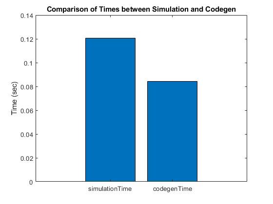
Compare Simulation and Codegen Performance (Optional)

You can evaluate the time taken to run the semantic segmentation network in both the simulation and codegen scenarios and plot the comparison using the following code.

codegenfHandle = @() networkPredict_mex(spectrogramInput{1});
% Evaluate the time taken for codegen 
codegenTime = timeit(codegenfHandle);
simulationfHandle = @() networkPredict(spectrogramInput{1}, networkFileName);
% Evaluate the time taken for simulation 
simulationTime = timeit(simulationfHandle);
% Plot performance comparison graph
figure(1);
% Create a vector with the simulation and codegen time values
timeValues = [simulationTime, codegenTime];
% Plot the bar graph
bar(timeValues);
% Add labels and a title
set(gca, 'XTickLabel', {'simulationTime', 'codegenTime'});
ylabel('Time (sec)');
title('Comparison of Times between Simulation and Codegen');

Further Exploration

The trained network in this example can distinguish between noise, LTE, NR, and unknown signals. To enhance the training data, create a trained network by referring to the Spectrum Sensing with Deep Learning to Identify 5G and LTE Signals example and generate more representative synthetic signals, or refer Capture and Label NR and LTE Signals for AI Training example to capture over-the-air signals and include these in the training set for more accurate signal identification.

You can also adjust the sample rate and center frequency or regenerate the training data and retrain the network to improve the identification of signals.

Supporting Functions

function I = helperSpecSenseSpectrogramImageFile(x,Nfft,sr,imgSize)
%   helperSpecSenseSpectrogramImageFile: Generate spectrogram image from baseband signal
%   I = helperSpecSenseSpectrogramImageFile(X,NFFT,SR,IMGSZ) calculates the
%   spectrogram of baseband signal X, using NFFT length FFT and assuming
%   sample rate of SR. 


window = hann(256);
overlap = 10;
% Generate spectrogram
[~,~,~,P] = spectrogram(x,window,overlap,...
  Nfft,sr,'centered','psd');

% Convert to logarithmic scale
P = 10*log10(abs(P')+eps);

% Rescale pixel values to the interval [0,1]. Resize the image to imgSize
% using nearest-neighbor interpolation.
im = imresize(im2uint8(rescale(P)),imgSize,"nearest");

% Convert to RGB image with parula colormap. 
I = im2uint8(flipud(ind2rgb(im,parula(256))));
end

function [net, networkFileName] = hLoadNetworkFromMATFile(baselineNetwork)
%   hLoadNetworkFromMATFile: Load the network MAT file based on the chosen baseline network.
%   [net, networkFileName] = hLoadNetworkFromMATFile(baselineNetwork) loads
%   the network into net and returns network file name.

    switch baselineNetwork
      case "custom"
        networkFileName = "specSenseTrainedNetCustom.mat";
      case "resnet18"
        networkFileName = "specSenseTrainedNetResnet18.mat";  
      case "resnet50"
        networkFileName = "specSenseTrainedNetResnet50.mat";    
      case "mobilenetv2"
        networkFileName = "specSenseTrainedNetMobileNetv2.mat";      
      otherwise
        error("Unknown baseline network: " + baselineNetwork)
    end
    net = load(networkFileName,'net');
    net = net.net;
end