Many times when ploting, we not only need to set the color of the plot, but also its
transparency, Then how we set the alphaData of colorbar at the same time ?
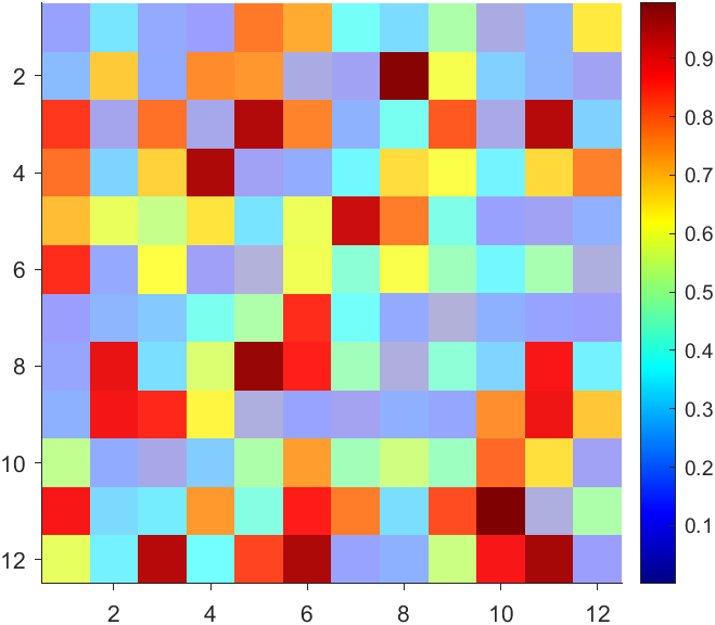
It seems easy to do so :
data = rand(12,12);
AData = rescale(- data, .3, 1);
imagesc(data, 'AlphaData',AData);
colormap(jet);
ax = gca;
ax.DataAspectRatio = [1,1,1];
ax.TickDir = 'out';
ax.Box = 'off';
CBarHdl = colorbar;
pause(1e-16)
CData = CBarHdl.Face.Texture.CData;
ALim = [min(min(AData)), max(max(AData))];
CData(4,:) = uint8(255.*rescale(1:size(CData, 2), ALim(1), ALim(2)));
CBarHdl.Face.Texture.ColorType = 'TrueColorAlpha';
CBarHdl.Face.Texture.CData = CData;
But !!!!!!!!!!!!!!! We cannot preserve the changes when saving them as images :
It seems that when saving plots, the `Texture` will be refresh, but the `Face` will not :
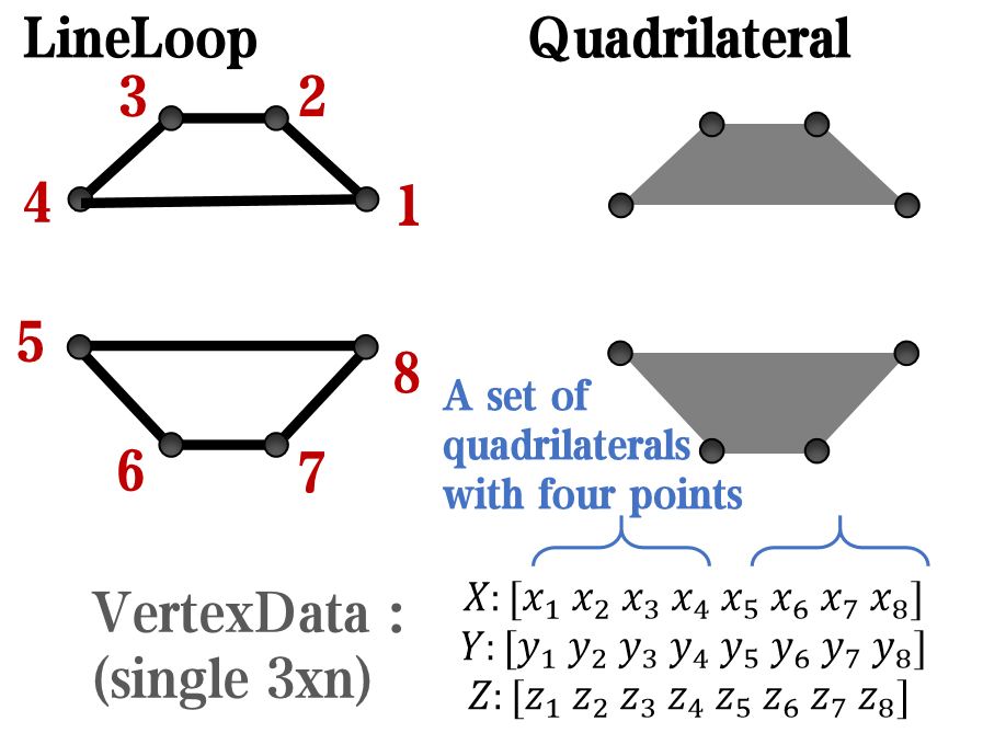
however, object Face only have 4 colors to change(The four corners of a quadrilateral), how
can we set more colors ??
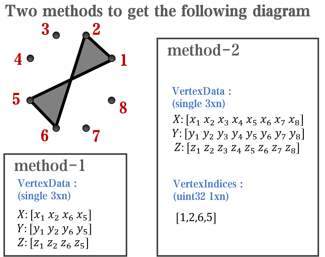
`Face` is a quadrilateral object, and we can change the `VertexData` to draw more than one little quadrilaterals:
data = rand(12,12);
AData = rescale(- data, .3, 1);
imagesc(data, 'AlphaData',AData);
colormap(jet);
ax = gca;
ax.DataAspectRatio = [1,1,1];
ax.TickDir = 'out';
ax.Box = 'off';
CBarHdl = colorbar;
pause(1e-16)
CData = CBarHdl.Face.Texture.CData;
ALim = [min(min(AData)), max(max(AData))];
CData(4,:) = uint8(255.*rescale(1:size(CData, 2), ALim(1), ALim(2)));
warning off
CBarHdl.Face.ColorType = 'TrueColorAlpha';
VertexData = CBarHdl.Face.VertexData;
tY = repmat((1:size(CData,2))./size(CData,2), [4,1]);
tY1 = tY(:).'; tY2 = tY - tY(1,1); tY2(3:4,:) = 0; tY2 = tY2(:).';
tM1 = [tY1.*0 + 1; tY1; tY1.*0 + 1];
tM2 = [tY1.*0; tY2; tY1.*0];
CBarHdl.Face.VertexData = repmat(VertexData, [1,size(CData,2)]).*tM1 + tM2;
CBarHdl.Face.ColorData = reshape(repmat(CData, [4,1]), 4, []);
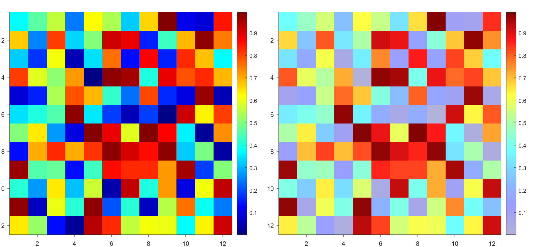
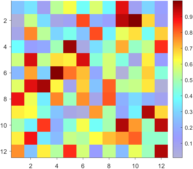
The higher the value, the more transparent it becomes
data = rand(12,12);
AData = rescale(- data, .3, 1);
imagesc(data, 'AlphaData',AData);
colormap(jet);
ax = gca;
ax.DataAspectRatio = [1,1,1];
ax.TickDir = 'out';
ax.Box = 'off';
CBarHdl = colorbar;
pause(1e-16)
CData = CBarHdl.Face.Texture.CData;
ALim = [min(min(AData)), max(max(AData))];
CData(4,:) = uint8(255.*rescale(size(CData, 2):-1:1, ALim(1), ALim(2)));
warning off
CBarHdl.Face.ColorType = 'TrueColorAlpha';
VertexData = CBarHdl.Face.VertexData;
tY = repmat((1:size(CData,2))./size(CData,2), [4,1]);
tY1 = tY(:).'; tY2 = tY - tY(1,1); tY2(3:4,:) = 0; tY2 = tY2(:).';
tM1 = [tY1.*0 + 1; tY1; tY1.*0 + 1];
tM2 = [tY1.*0; tY2; tY1.*0];
CBarHdl.Face.VertexData = repmat(VertexData, [1,size(CData,2)]).*tM1 + tM2;
CBarHdl.Face.ColorData = reshape(repmat(CData, [4,1]), 4, []);
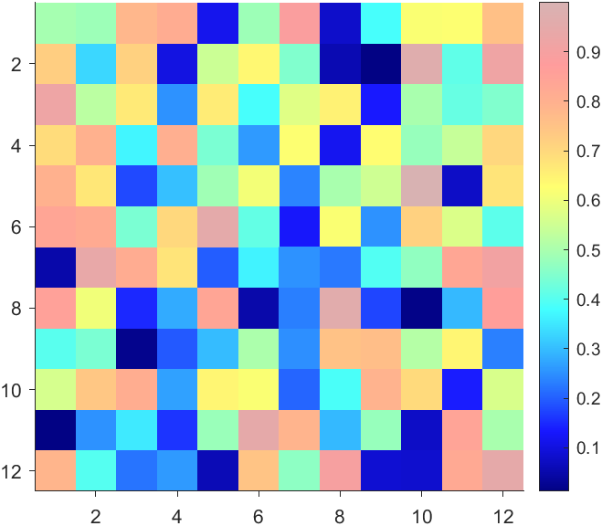
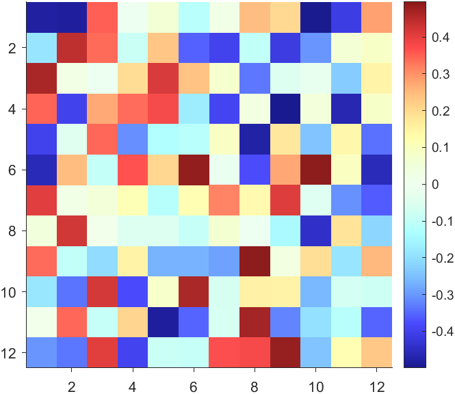
More transparent in the middle
data = rand(12,12) - .5;
AData = rescale(abs(data), .1, .9);
imagesc(data, 'AlphaData',AData);
colormap(jet);
ax = gca;
ax.DataAspectRatio = [1,1,1];
ax.TickDir = 'out';
ax.Box = 'off';
CBarHdl = colorbar;
pause(1e-16)
CData = CBarHdl.Face.Texture.CData;
ALim = [min(min(AData)), max(max(AData))];
CData(4,:) = uint8(255.*rescale(abs((1:size(CData, 2)) - (1 + size(CData, 2))/2), ALim(1), ALim(2)));
warning off
CBarHdl.Face.ColorType = 'TrueColorAlpha';
VertexData = CBarHdl.Face.VertexData;
tY = repmat((1:size(CData,2))./size(CData,2), [4,1]);
tY1 = tY(:).'; tY2 = tY - tY(1,1); tY2(3:4,:) = 0; tY2 = tY2(:).';
tM1 = [tY1.*0 + 1; tY1; tY1.*0 + 1];
tM2 = [tY1.*0; tY2; tY1.*0];
CBarHdl.Face.VertexData = repmat(VertexData, [1,size(CData,2)]).*tM1 + tM2;
CBarHdl.Face.ColorData = reshape(repmat(CData, [4,1]), 4, []);
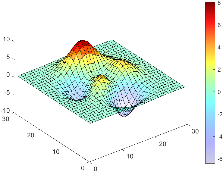
The code will work if the plot have AlphaData property
data = peaks(30);
AData = rescale(data, .2, 1);
surface(data, 'FaceAlpha','flat','AlphaData',AData);
colormap(jet(100));
ax = gca;
ax.DataAspectRatio = [1,1,1];
ax.TickDir = 'out';
ax.Box = 'off';
view(3)
CBarHdl = colorbar;
pause(1e-16)
CData = CBarHdl.Face.Texture.CData;
ALim = [min(min(AData)), max(max(AData))];
CData(4,:) = uint8(255.*rescale(1:size(CData, 2), ALim(1), ALim(2)));
warning off
CBarHdl.Face.ColorType = 'TrueColorAlpha';
VertexData = CBarHdl.Face.VertexData;
tY = repmat((1:size(CData,2))./size(CData,2), [4,1]);
tY1 = tY(:).'; tY2 = tY - tY(1,1); tY2(3:4,:) = 0; tY2 = tY2(:).';
tM1 = [tY1.*0 + 1; tY1; tY1.*0 + 1];
tM2 = [tY1.*0; tY2; tY1.*0];
CBarHdl.Face.VertexData = repmat(VertexData, [1,size(CData,2)]).*tM1 + tM2;
CBarHdl.Face.ColorData = reshape(repmat(CData, [4,1]), 4, []);


 $ is the unknown displacement of the oscillator occupying the n-th position of the lattice, and
 and
and  , that is,
 for the one-dimensional discrete Laplacian
 . We consider spatially extended initial conditions of the form:
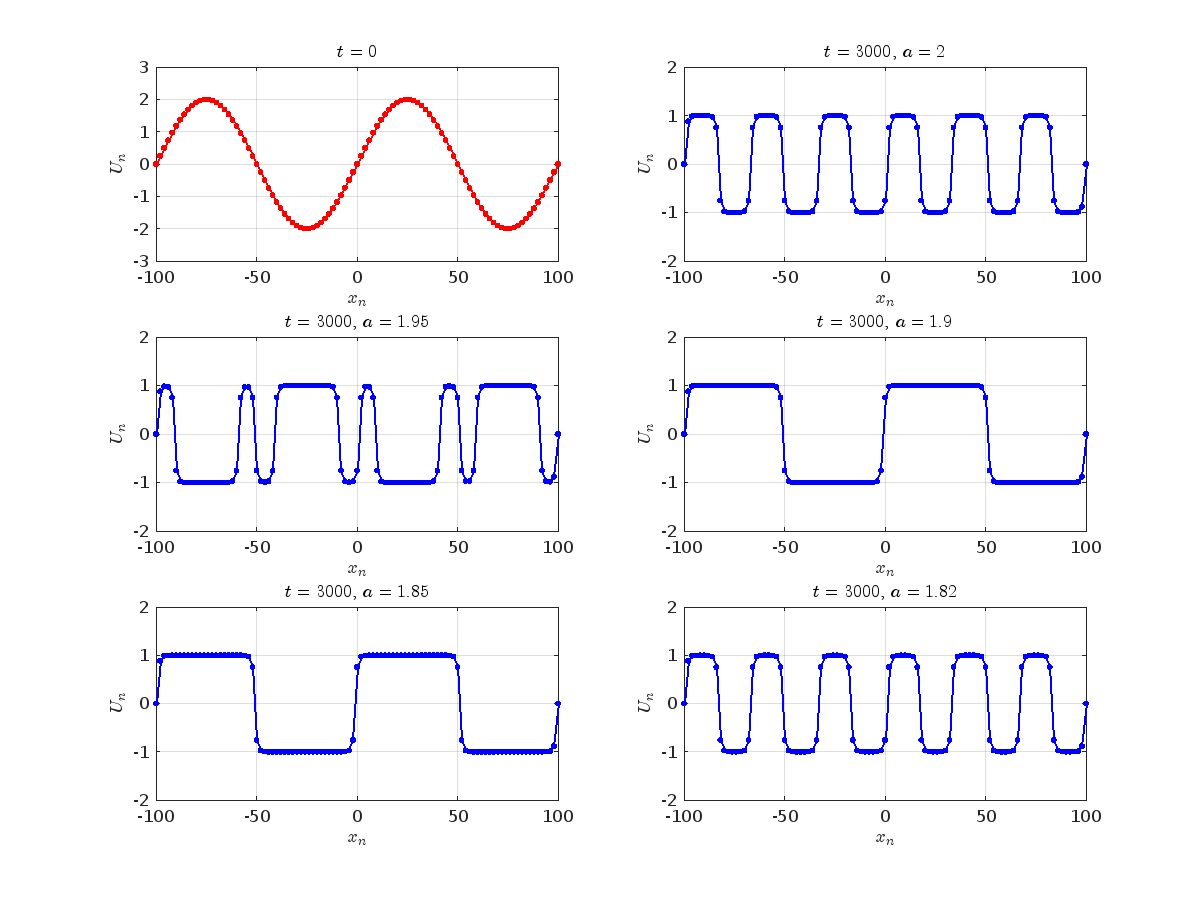
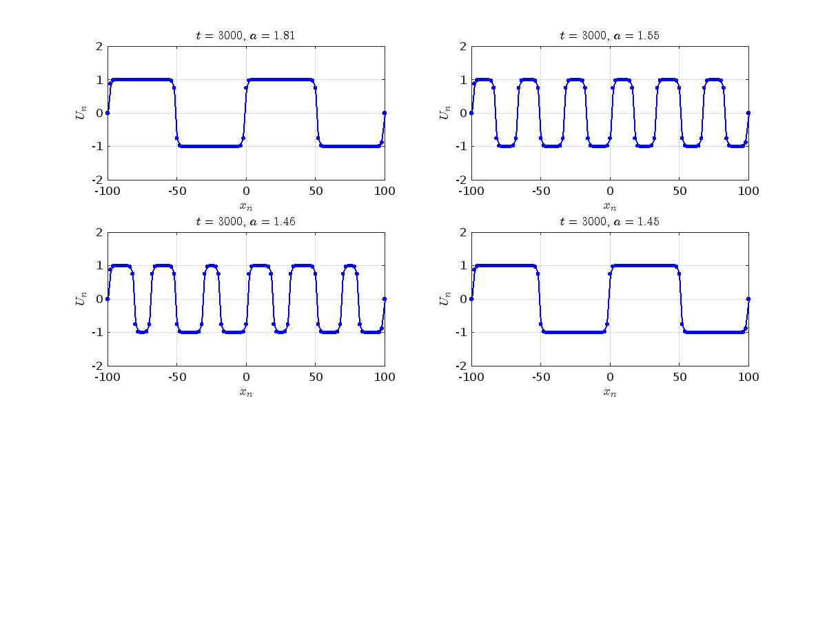
 where the dynamics appear in the first image of the third row, we observe convergence to a non-linear equilibrium point of branch
  respectively, converges to a non-linear equilibrium point of branch
  and energy