Market-Implied Systemic Risk in a Banking System
The Bank of England measures systemic risk within a banking system based on market-implied expected losses. Ken Deeley of MathWorks presents joint work with Somnath Chatterjee of the Centre for Central Banking Studies at the Bank of England using a structural credit risk model. The model, developed using MATLAB® and Financial Toolbox™, is based on a jump diffusion process, which defines the probability of default based on the risk-adjusted balance sheet of banks whose assets are stochastic and may be above or below promised payments on its debt obligations. Using this framework, they estimate implied asset values and expected losses of individual banks. They then develop a model to estimate the joint-default risk of multiple banks falling into distress as a portfolio of individual market-implied expected losses using generalized extreme value (GEV) analysis and a multivariate copula as a dependence measure.
Published: 16 Nov 2022
My name is Ken Deeley. I'm an application engineer at MathWorks. And as Rich mentioned, this is a presentation on some joint work that we've done with the Bank of England. The topic is "Market-implied systemic risk in a banking system."
So, since Somnath is not here, I'll just introduce him. Somnath is a senior economist and advisor at the Centre for Central Banking Studies at the Bank of England. The CCBS is responsible for disseminating research, code, and models from the Bank of England to other central banks around the world. They did put a high priority on education of central bankers. So communicating and disseminating research is a top priority.
And code and models that are developed at the CCBS, these can be written in any language. Primary languages are MATLAB or EViews, Stata, and Python. We've also been working with Somnath as part of collaboration with MathWorks development, as well. So, some of the more recent features that you might have seen in different financial toolboxes, these have been developed in collaboration with Somnath and others at the Bank of England.
So, to give a couple of examples, jump-diffusion models were introduced in the Financial Toolbox, back in 20a. And there are ongoing discussions regarding quantile regression in The statistics Toolbox as well. So I think this highlights a great opportunity. If anyone has feedback, this is something that you can share directly with MathWorks and also get in touch with MathWorks' development team, as well, to provide your feedback on things that should be included in the toolboxes.
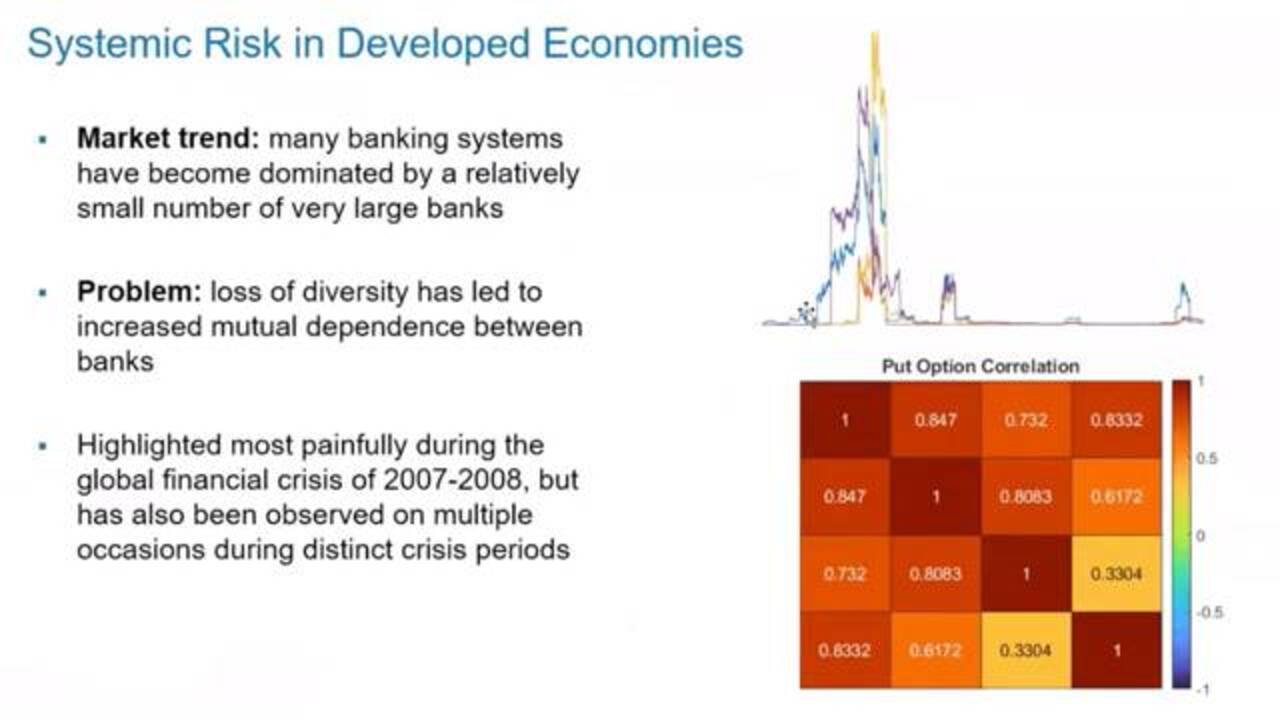
So, switching to the topic of the presentation-- this is all about assessing systemic risk, mainly in developed economies. As you all know, in recent years banking systems have become dominated by a fairly small number of large banks, especially the developed economies. That's kind of a general market trend. And one of the issues with this is that some diversity has been lost.
And because that diversity has been lost, it means that there's increased dependency, mutual dependency, between banks within the banking system. Clearly this is something that caused a lot of pain and stress during the global financial crisis, back in 2007-2008, but since then this systemic risk, which is caused by mutual dependencies between institutions, this has also been observed on other crisis periods as well.
So part of the motivation for doing this sort of work is to try and assess whether early-warning systems could be developed. Sometimes these are referred to as "black swans," these crisis periods, referring to the presence of some unexpected or extreme event that nobody was able to predict or foresee. And also another motivation, as well as trying to get some insight into when these things are going to happen and what their duration is and what their impacts will be, another important consideration is whether independent analysts could develop these types of models based on freely available market data.
So the idea is, this shouldn't just be something that only central bankers can do or only people working in high-profile financial institutions can do. Ideally, this is something that would be open to citizen analysts or citizen data scientists who can work with freely available data and maybe help to predict these types of things.
And we have looked at this sort of analysis before. A few years ago, back in 2018, 2019, we looked at a similar approach about working with company data-- taking essentially market-capitalization time series and then trying to model market-implied value of a particular company, along with other quantities such as the debt and the leverage, default probability, and things like that. So this talk is very much related to this previous work but is mainly focused on looking at mutual dependencies between banks rather than looking at individual companies.
So what data are we using, in this model? It's all put options. These time series that you saw here, on the previous slide, these are all put options for banks. This is the overall correlation matrix between those four sets of put options. You can see, the correlation is very, very high.
What is a put option? I'm sure most of you are familiar with put options already, but I'll just run through some key aspects of what put options are and why they're useful for this type of modeling. So a put option is essentially a bet that the future price of an asset is going to fall. So you would tend to buy a put option if you're feeling a bit bearish-- if you have a pessimistic outlook. If you think the future asset price is going to drop, then it makes sense to buy a put option.
And some key aspects of put options that make them useful, in this context, is, if you're studying an asset, such as a bank, and that underlying asset starts to lose value, we expect the put-option values to increase because the payoff of the option also increases.
In terms of volatility, whenever you have increased volatility this increases the value of the put option, essentially because there's more downside risk. So if you have increased volatility, you have increased downside risk and therefore an increased payoff, potential payoff, for the put option.
That's actually true for call options, as well, using the same arguments that the volatility increases, then the upside risk also increases, and therefore the value of the call option increases, as well. And also-- and this is very important, from a crisis-analysis point of view-- put-option values tend to have a spike, and if there's some underlying market sentiment that the assets-- the bank, in this case-- is in trouble.
So if you look back at the last 15, 20 years or so of put-option data for these four banks, you can see these spikes in the put-option values. These tend to correspond to the different crisis periods that have occurred during that time frame. So obviously the global financial crisis, as we mentioned before, that's the biggest peak, here. But also, to a lesser extent, you can see smaller crises, as well. So the eurozone sovereign debt crisis, back in 2011-2012, the EU referendum-- Brexit referendum-- back in 2016, and also the impact of COVID-19 in early 2020 and going into 2021.
And another key thing to observe here is that some of these crises are kind of internal to the banking system. You could argue that the global financial crisis and the Eurozone crisis are both examples where the responsibility, if you like, belongs to the financial system, whereas some of these shocks are exogenous in nature, like the EU referendum. And clearly COVID-19 is an external shock. But both internal and external shocks are reflected in the values of the put options.
In terms of requirements for this model, what we want is to have a single risk index. So the objective here is to take this put-option data, representing four different banks in the system, and then come up with a single risk index that quantifies the overall systemic risk, the implied risk, in some way. And from that index, we should be able to produce one-step-ahead forecasts.
I already mentioned the two different types of shocks that can occur-- the endogenous or in-system shocks, as well as the exogenous or out-of-system shocks. And what you can see, by studying the data, is that these shocks tend to have a standard pattern associated with them. At the start of the crisis period, there's this very, very rapid increase in the put-option values, representing this sort of market sentiment-- or "panic," as I've called it in the slide here.
And then, after a while, there's kind of a plateau period of people coming to terms with what's happened, coming to terms with the crisis-- the acceptance or absorbance period. And then that's then followed by some return to what we might call "normal" conditions, as people start to identify solutions to the underlying nature of the crisis.
So that sort of standard psychological profile, if you like, that's something that we want to capture in the model. And that's something that's exhibited by all four shocks that are represented in that data set.
For the rest of the talk, I'll focus on the details of the model that we've constructed and put together. There are several different modeling steps. First of all, the module itself is fitted on a rolling window basis. The input data is the put options, as we discussed before. And the first thing that we're modeling is the autocorrelation within the put options.
So it's very much the case that the put option at time t depends on the put option at time t minus 1. So there's a strong dependency on what the previous value of the put option was. And we capture that with the standard ARIMA model-- just a simple autoregressive model with one term.
And what we find with this data is that, in most of the rolling windows, in most of the moving windows, in the data set, that autoregressive coefficient-- the alpha, in this equation here-- that's actually quite close to 1, which implies that the put options behave quite closely to how a random walk behaves, as you might expect. However it's not a perfect random walk, by any means. And the reason for that is, when you start to enter a crisis period, the jumps in this process become unusually large.
So, for a standard random walk, you would expect the jumps-- the epsilon t, in this expression here-- these would be normally distributed. And therefore the number of extreme jumps would be relatively low and measurable. But that's actually not the case in the data. When you start to enter a crisis period, the jumps get very large. They also don't follow a normal distribution, as well.
So that leads us to the next modelting step, and that's to somehow take into account the non-normal nature of these jumps. And this is where we're using something called "extreme value theory," which some of you might be familiar with. This is a kind of general area of statistics and risk management where you're interested in modeling the presence of rare or extreme or unusual events.
This is quite often used in applications such as climate risk, where you're interested in measuring and modeling things like flood risk, storm risk, damage from sea-level rise and sea flooding-- things like that. So you're interested in modeling the frequency of those events but also the impact of those events, as well.
So, how often is this event likely to happen? And also, if it does happen, what's the expected level of damage that will occur? This can be applied in quite a wide variety of situations, including this market-based, implied-risk application that we're talking about just now.
The probability distribution that we're using in MATLAB is the Generalized Extreme Value, or GEV, distribution. That has three parameters, two of which are fairly standard-- the location and scale parameters that most parametric-probability distributions used in this area have. However, there is a third parameter, as well, the shape parameter, and that's what makes this distribution quite interesting and also suitable for use in extreme-value applications.
This animation that's playing down here, this represents what happens to the density function as you change that shape parameter. That has the biggest impact on changing what this distribution looks like. And it's quite powerful. You can use it to model the tail of a probability distribution, which has potentially quite a strange shape. And this is something that's quite common in lots of financial time series, especially ones that contain the presence of these large jumps and large extreme values.
This is fine in theory. In practice, there are, again, some more issues involved with actually fitting this. It is actually quite an unstable distribution to fit. It doesn't always converge.
So, to work around that in MATLAB, it's possible to extend the number of iterations used in the optimization routine. For example, you can just let the solver run a little bit longer and see if that converges. It's also possible to use techniques such as global optimization, available in the Global Optimization Toolbox in MATLAB. And that can help you to find an optimum set of parameters for this distribution, as well.
We also carefully validate each fit, as well. We don't just assume that the data follows that distribution. We also validate it, using hypothesis testing. That's the Kolmogorov-Smirnov test, which is available in Stats Toolbox .
In very extreme cases where this doesn't actually converge at all, we revert back to using the empirical CDF of the data. And that's something that's guaranteed to at least produce a reasonable fit in that time period. The empirical CDF doesn't help to explain the extreme events, but it's a useful backup if this GEV fit fails to converge. So the overall model here is a combination of generalized extreme value fits plus a few empirical CDFs corresponding to the windows where this fails to converge.
So at this point, we've modeled each of the banks within the banking system individually. What we haven't done is captured how the banks relate to each other. So we mentioned, near the start of the talk, that one of the main reasons for doing this is to try and capture the very high correlation and dependency between the banks that we observe in crisis periods. Steps 1 and 2 deal with banks individually. Step three brings those individual pieces, those marginal models, together, in order to capture the dependencies between the banks.
So once the marginal distributions have been fitted-- that's steps 1 and 2-- we then bring those marginals together, using a copula. The copulas have been criticized quite a lot, especially during the financial crisis, for not capturing some of the key aspects of the data that was observed. That criticism was mainly aimed at people using Gaussian copulas not checking that the assumptions were satisfied.
So in this case, we're using a t copula, available in MATLAB, rather than a Gaussian copula. You can see the difference, roughly, in these two plots on the top right, here. These both show two-dimensional copulas.
You can see the t copula actually does quite a good job of picking up some of the tails, represented at the top left and the bottom-right corners of this plot here. And those areas correspond to points where one bank has a low value and the other bank has a high value. And that can sometimes happen.
It is true that the put options of the banks are highly correlated, and they all move together, but they don't necessarily all jump at exactly the same time. And you can see that in some of these plots here. You can see that bank 1, for example, has jumped up before bank 2 jumps, and then bank 2 jumps, and it jumps to a higher point than bank 1. To capture that effectively in a model, you really need to use a copula that can also handle these tail events
In the corners, here. Now, these pictures that I've drawn here, these are obviously two-dimensional. But one of the benefits of computers is they extend to any number of dimensions. So in this case, we had four banks, and therefore we'd be fitting a four-dimensional t copula.
This animation here is showing what happens when you change the number of degrees of freedom in the copula. And that's something that the t distribution gives you flexibility over. You don't have that extra parameter when you're fitting a Gaussian copula. And this is another advantage of using the t distribution here, is, you can change that degrees of freedom and potentially model quite a wide variety of different shapes, represented by the different shapes shown in this animation.
Again, there's one issue with fitting this, and that's, in the very, very extreme periods, the correlation between the banks and the system, that increases very rapidly, and the correlation matrix actually approaches a matrix of ones-- which is rank-deficient. And that causes the convergence process to fail.
So in that situation, at the very top of the crisis, we just simply replace the correlation matrix with the matrix of ones and assume that the system has kind of broken down.
Right. So that's the three main modeling steps. Once you've got the copula in place, it's then possible to use the copula to perform Monte Carlo simulation. So we back-transform the copula samples back into the put-option domain and then calculate some standard risk metrics, like value of risk and expected shortfall.
In terms of results, we find that this model does quite a good job of responding to the different crisis periods. You can see the input data at the top, here. This is the put-option values and then the output data from the model, which, we're calling this "systemic risk index." This is shown on the bottom plot, here. And it seems to be quite a good job of capturing the four different crises relatively well.
The other important thing that I already mentioned is that this module is constructed from just some simple market data. The starting point is some put options. If you had a model for put options, you could obviously use that, as well, or you could just simply use observed put-option values from the market.
So, to summarize this, we've written a paper together, which is in process of being submitted to a journal and will also be having to share the code methodology, as well, with other central banks. All right. So I think that's everything from me. So-- happy to answer any questions that people have. Thanks very much for listening.
Featured Product
MATLAB
Up Next:

Related Videos:


Seleccione un país/idioma
Seleccione un país/idioma para obtener contenido traducido, si está disponible, y ver eventos y ofertas de productos y servicios locales. Según su ubicación geográfica, recomendamos que seleccione: United States.
También puede seleccionar uno de estos países/idiomas:
América
- América Latina (Español)
- Canada (English)
- United States (English)
Europa
- Belgium (English)
- Denmark (English)
- Deutschland (Deutsch)
- España (Español)
- Finland (English)
- France (Français)
- Ireland (English)
- Italia (Italiano)
- Luxembourg (English)
- Netherlands (English)
- Norway (English)
- Österreich (Deutsch)
- Portugal (English)
- Sweden (English)
- Switzerland
- United Kingdom (English)