Optimize Enclosure for Edge-Coupled Filter Using SADEA Optimizer

Since R2026a

This example shows how to optimize the enclosure for an edge-coupled filter using the SADEA optimizer. The goal is to minimize enclosure-induced resonances that degrade filter performance. SADEA is a surrogate-assisted optimization method that uses mathematical models to approximate expensive electromagnetic (EM) simulations, significantly improving computational efficiency. It is particularly effective when the design space contains a small number of variables.

The example requires the Integro-Differential Modeling Framework for MATLAB add-on. To enable the add-on:

1. In the Home tab in the Environment section, click Add-Ons and open the add-on explorer.

2. Search for Integro-Differential Modeling Framework for MATLAB and click Install

3. To verify if the download is successful, run matlab.addons.installedAddons in your MATLAB® Command Window.

Create Coupled-Line Filter

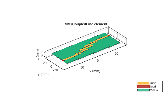
Use the design function of the filterCoupledLine object to design the filter at 3 GHz.

coupledfilter = design(filterCoupledLine,3e9);
figure
show(coupledfilter)

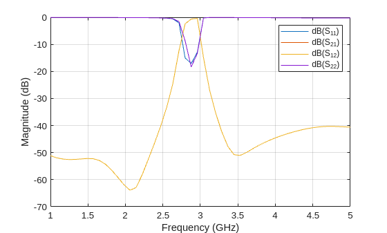
Plot Reflection Coefficient

The filterCoupledLine object uses method of moments (MoM) as the default solver. Plot the filter’s reflection coefficient from 1 to 5 GHz with a 50-ohm reference impedance.

sp = sparameters(coupledfilter,linspace(1e9,5e9,50));
figure
rfplot(sp);

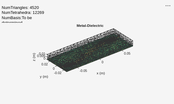
Save mesh parameters used for S-parameter calculation.

m = mesh(coupledfilter)

m = 
  MeshReader with properties:

                Points: [3×1722 double]
             Triangles: [4×1966 double]
            Tetrahedra: [4×4854 double]
         MaxEdgeLength: 0.0054
         MinEdgeLength: 0.0033
            GrowthRate: 0.1200
    MinimumMeshQuality: 0.0615
              MeshMode: 'auto'

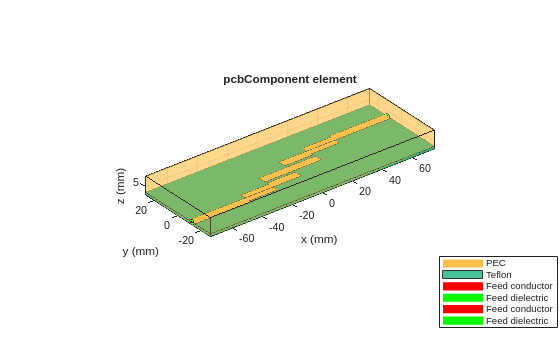
Convert Filter Object to pcbComponent

Convert the filter object to a pcbComponent object and set the SolverType property to 'FEM'.

p = pcbComponent(coupledfilter); 
p.SolverType= 'FEM';
p.IsShielded = true; % Enable the enclosure
p.Shielding.Height = 11.4e-3; % Height of the enclosure

Offset the center of the enclosure in the z-direction to ensure that it is positioned above the z = 0 plane.

p.Shielding.Center = [0 0 0.5*p.Shielding.Height];

Add RF connector to the pcbComponent object.

c = RFConnector(...
    InnerRadius=4.39384e-4,...
    OuterRadius=coupledfilter.Height,...
    EpsilonR=coupledfilter.Substrate.EpsilonR,...
    PinLength=1e-4);
p.Connector = c;

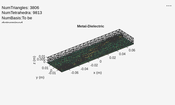
Visualize the coupled-line filter with enclosure.

figure
show(p)

Apply Mesh and Perform S-parameters Frequency Sweep

Use the sparameters function to compute the S-parameters of the edge-coupled filter in a shielded rectangular cavity. Using the same mesh settings as in the MoM simulation, sweep the frequency from 1 to 5 GHz to plot the results.

mesh(p,MaxEdgeLength=m.MaxEdgeLength,MinEdgeLength=m.MinEdgeLength,GrowthRate=m.GrowthRate);

spar2 = sparameters(p,linspace(1e9,5e9,50));
figure
rfplot(spar2)
legend(Location="southwest")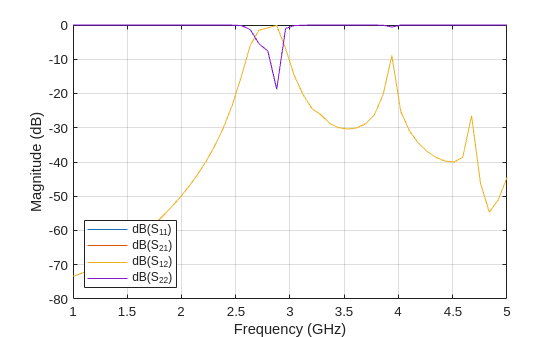

From the plot, the overall trend matches the case without a shield. However, box resonances appear around 3.8 GHz and 4.7 GHz.

Optimize Filter to Remove Unwanted Resonances

Use the OptimizerSADEA object to optimize this filter. This object provides access to the SADEA optimizer in Antenna Toolbox™. Initialize the optimizer by specifying the lower and upper bounds of the design variables. Then, use the custom evaluation function defined in the Supporting Functions section to set the optimization objective. Run optimizeWithPlots function with 15 iterations to perform the optimization.

In this example, the design variable is GroundPlaneWidth. The calculateUnwantedResonances function uses this variable to control the filter ground plane width. Write the evaluation function to measure any sharp deviations like peaks or nulls from the smooth curve. Because the enclosure dimensions in the x‑ and y‑directions match the ground plane size (only the height differs), GroundPlaneWidth indirectly determines the enclosure size.The chosen range for GroundPlaneWidth is 35 mm to 70 mm.

s = OptimizerSADEA([35e-3;70e-3]);
s.CustomEvaluationFunction = @calculateUnwantedResonances;
s.EnableLog = true;
optimize(s,15);

Iteration: 1,  Best: 2.029370 
Iteration: 2,  Best: 2.029370 
Iteration: 3,  Best: 2.029370 
Iteration: 4,  Best: 2.029370 
Iteration: 5,  Best: -0.952447 
Iteration: 6,  Best: -14.686389 
Iteration: 7,  Best: -14.686389 
Iteration: 8,  Best: -14.686389 
Iteration: 9,  Best: -15.501113 
Iteration: 10,  Best: -15.501113 
Iteration: 11,  Best: -15.501113 
Iteration: 12,  Best: -15.501113 
Iteration: 13,  Best: -15.501113 
Iteration: 14,  Best: -15.501113 
Iteration: 15,  Best: -15.501113 
Iteration: 16,  Best: -15.501113 

Use the getBestMemberData function to fetch the optimized values for the design variables.

bestData = getBestMemberData(s);
optimized_values = bestData.member;

Apply the optimized values to the evaluation function to get the filter object.

[~,p] = calculateUnwantedResonances(optimized_values)

p = 
  pcbComponent with properties:

              Name: 'Coupled Line Filter'
          Revision: 'v1.0'
        BoardShape: [1×1 antenna.Rectangle]
    BoardThickness: 0.0016
            Layers: {[1×1 antenna.Polygon]  [1×1 dielectric]  [1×1 antenna.Rectangle]}
        FeedFormat: 'FeedLocations'
     FeedLocations: [2×4 double]
      ViaLocations: []
       ViaDiameter: []
         Conductor: [1×1 metal]
              Tilt: 0
          TiltAxis: [0 0 1]
              Load: [1×1 lumpedElement]
        SolverType: 'FEM'
        IsShielded: 1
         Connector: [1×1 RFConnector]
         Shielding: [1×1 shape.Box]

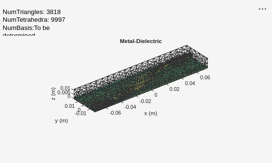
figure
show(p)
title("Optimized EdgeCoupledFilter")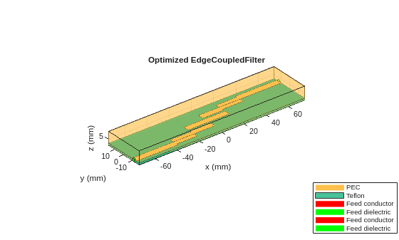

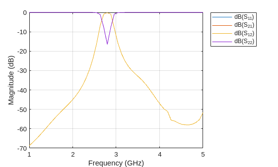
Plot Reflection Coefficient of Optimized Filter

Plot the reflection coefficient of the optimized filter from 1 to 5 GHz with a 50-ohm reference impedance. Observe that, most unwanted resonances are filtered out compared to the initial design.

freq = 1e9;
freqRange = linspace(freq*1, freq*5, 50);
sparam = sparameters(p,freqRange);
rfplot(sparam);

Get Optimization Data

Get the iteration data using the getIterationData function. The column in the IterationMembers variable represents the GroundPlaneWidth design variable values for different iterations.

iterData = getIterationData(s);
IterationMembers = iterData.members

IterationMembers = 15×1

    0.0506
    0.0488
    0.0502
    0.0356
    0.0351
    0.0354
    0.0357
    0.0350
    0.0359
    0.0365
    0.0350
    0.0353
    0.0353
    0.0350
    0.0354
      ⋮

Get the surrogate model data (initial population) using getInitializationData function. The column in the InitializationMembers variable represents the GroundPlaneWidth design variable values for initial sampling.

initialData = getInitializationData(s);
InitializationMembers = initialData.members

InitializationMembers = 30×1

    0.0371
    0.0466
    0.0386
    0.0407
    0.0637
    0.0619
    0.0517
    0.0695
    0.0595
    0.0385
    0.0434
    0.0676
    0.0490
    0.0472
    0.0546
      ⋮

Check if the algorithm has converged.

convergence = isConverged(s)

convergence = logical
   0

Get the number of times the evaluation function has been evaluated.

NumberOfEvaluations = getNumberOfEvaluations(s)

NumberOfEvaluations = 
45

Supporting Function

This section defines the calculateUnwantedResonances function, which sets the optimization objective. It is designed to detect sharp deviations (peaks or nulls) from a smooth response. The function removes peaks and valleys, interpolate a smooth curve with the remaining data, and then aggregate the differences between the smooth curve and the original data to quantify the deviations.

function [fitness,p] = calculateUnwantedResonances(designVariables)
    try
        % Design coupled line filter object at 3 GHz.
        coupledfilter = design(filterCoupledLine,3e9);
        % Assign the design variable from optimization run to the object.
        coupledfilter.GroundPlaneWidth = designVariables;
        % Convert the filterCoupledLine object to a pcbComponent to use FEM solver.
        p = pcbComponent(coupledfilter);
        p.SolverType= 'FEM';
        p.IsShielded = true;
        p.Shielding.Height = 11.4e-3;
        % Offset center of the shielding in the z-direction to ensure it lies above the z = 0 plane.
        p.Shielding.Center = [0 0 0.5*p.Shielding.Height];
        % Add RF connector to the pcbComponent.
        c = RFConnector(...
            InnerRadius=4.39384e-4,...
            OuterRadius=coupledfilter.Height,...
            EpsilonR=coupledfilter.Substrate.EpsilonR,...
            PinLength=1e-4);
        p.Connector = c;

        % Use the same mesh settings as in the MoM simulation; sweep the
        % frequency from 1 to 5 GHz.
        mesh(p,MaxEdgeLength = 0.0054,MinEdgeLength = 0.0033,GrowthRate = 0.12);
        freqList = linspace(1e9,5e9,50);        
        spar = sparameters(p,freqList);
        % Get the transmission results from sparameters as vector.
        sp12 = reshape(20*log10(abs(spar.Parameters(1,2,:))),[],1);
        % Find the peak locations in the data.
        [~,locs] = findpeaks(sp12);
        % Find the valley locations in the data.
        [~,vlocs] = findpeaks(-1*sp12);
        % Merge both peak and valley locations.
        tlocs = [locs;vlocs];
        % Remove peak and valley data to prepare for interpolation.
        filteredFreq = freqList;
        filteredData = sp12;
        filteredData(tlocs)=[];
        filteredFreq(tlocs)=[];
        % Linearly interpolate filtered data to make smooth curve without peaks and
        % valleys.
        interPolatedData = interp1(filteredFreq,filteredData,freqList,'linear');
        % Compute the deviation of smooth curve from original curve.
        delta = interPolatedData - sp12';
        % Aggregate the deviation to quantify the total deviation.
        aggregate_deviation = sum(abs(delta)); % Value increases to be more positive;
        % Optimizer tries to reduce this value and bring it closer to
        % zero over iterations.

        % Get the return loss results from sparameters as vector.
        sp11 = reshape(20*log10(abs(spar.Parameters(1,1,:))),[],1);
        % Find locations for valleys in return loss data.
        [valleys,locs] = findpeaks(-1*sp11);
        
        % Identify the region of interest in pass band by removing
        % the stop band.
        lower_stop_band = freqList < 2.5e9;
        upper_stop_band = freqList > 3.5e9;
        % Get the IDs of the region of interest by negating the stopband.
        reqID = find(~(lower_stop_band | upper_stop_band));
        % Find valleys in the return loss graph. The objective is to
        % increase return loss or make the valley deeper near design frequency.
        valleyID = find(ismember(locs,reqID));
        valleyValue = -1*sum(valleys(valleyID)); % Better the return loss, deeper the value.
        % Optimizer tries to reduce this value and make it more negative.
        
        % Add both objectives reducing deviations and improving return
        % loss to get the total fitness.
        if ~isempty(valleyValue)
            fitness = aggregate_deviation + valleyValue;
        else
            fitness = aggregate_deviation;
        end
    catch
        % Use high penalty value to handle errors during objective evaluation.
        fitness = 1e6;
    end
end

Conclusion

This example builds and analyzes the basic structure of the edge-coupled filter. Using a SADEA optimizer object, you optimize the filter to maximize the return loss in the passband. The optimized design shows improved return loss compared to the initial prototype, as unwanted resonances are effectively reduced. The return loss of the optimized filter remains below –10 dB across the passband.