Log IQ Samples and Visualize in Signal Analyzer

This example shows how to log, visualize, and analyze in-phase and quadrature (IQ) samples at the nodes in a Bluetooth® low energy (LE) and WLAN coexistence scenario.

Using this example, you can:

1. Create a Bluetooth LE-WLAN coexistence scenario consisting of a Central node, a Peripheral node, an access point (AP), and a station (STA).

2. Add On-Off application traffic between the nodes.

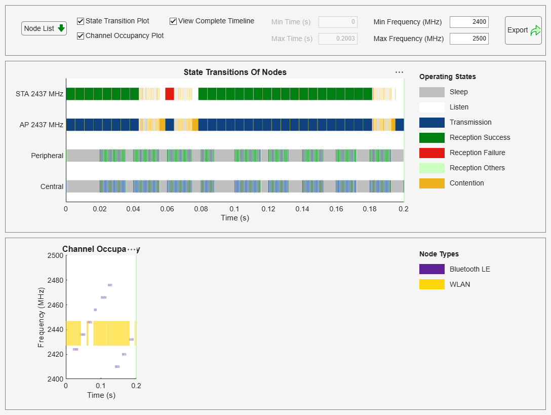
3. Simulate the scenario, and visualize the state transitions and channel occupancy of the nodes.

4. Log IQ samples at the nodes.

5. Visualize the IQ samples in the Signal Analyzer app, and analyze the results.

Set the random number generator to 1 to ensure the repeatability of results. The seed value controls the pattern of random number generation. Initializing the random number generator using the same seed ensures the same result. To improve the accuracy of your simulation results, after running the simulation, you can change the seed value, run the simulation again, and average the results over multiple simulations.

rng(1,"combRecursive")

Initialize the wireless network simulator.

networkSimulator = wirelessNetworkSimulator.init;

Create Bluetooth LE Nodes and Add Traffic

Create a Bluetooth LE Central node and a Peripheral node, specifying their names and positions (in meters).

centralNode = bluetoothLENode("central",Name="Central", ...
    Position=[0 0 0]);          % In x-, y-, and z-coordinates
peripheralNode = bluetoothLENode("peripheral",Name="Peripheral", ...
    Position=[1 0 0]);          % In x-, y-, and z-coordinates

Create a default Bluetooth LE link layer (LL) connection configuration object. Configure the LL connection between the Central and Peripheral nodes.

cfgConnection = bluetoothLEConnectionConfig;
configureConnection(cfgConnection,centralNode,peripheralNode);

Create and configure On-Off application traffic, specifying the data rate (in Kbps), packet size (bytes), On state and Off state duration (in seconds). Add application traffic at the Central node to Peripheral node.

LETraffic = networkTrafficOnOff(DataRate=200,PacketSize=27,OnTime=inf);
addTrafficSource(centralNode,LETraffic,DestinationNode=peripheralNode)

Create WLAN Nodes and Add Traffic

Configure a WLAN node as an AP by specifying the operating mode and type of interference modeling. Create a WLAN AP from the specified configuration, specifying the name, position (in meters), MAC frame abstraction, and PHY abstraction method.

accessPointCfg = wlanDeviceConfig(Mode="AP",BandAndChannel=[2.4 6],InterferenceModeling="overlapping-adjacent-channel");
accessPointNode = wlanNode(Name="AP",Position=[0 10 0],DeviceConfig=accessPointCfg,MACModel="full-mac",PHYModel="full-phy");

Configure a WLAN node as an STA by specifying the operating mode and type of interference modeling. Create a WLAN STA from the specified configuration, specifying the name, position (in meters), MAC frame abstraction method, and PHY abstraction method.

stationCfg = wlanDeviceConfig(Mode="STA",BandAndChannel=[2.4 6],InterferenceModeling="overlapping-adjacent-channel");
stationNode = wlanNode(Name="STA",Position=[5 0 0],DeviceConfig=stationCfg,MACModel="full-mac",PHYModel="full-phy");

Associate the STA node with the AP node.

associateStations(accessPointNode,stationNode)

Create and configure On-Off application traffic, specifying the data rate (in Kbps), and packet size (bytes). Add the application traffic at the AP node to the STA node.

wlanTraffic = networkTrafficOnOff(DataRate=10e6,PacketSize=1500,OnTime=inf);
addTrafficSource(accessPointNode,wlanTraffic,DestinationNode=stationNode)

Add Nodes to Simulator

Add all the nodes to the wireless network simulator.

addNodes(networkSimulator,[centralNode peripheralNode])
addNodes(networkSimulator,[accessPointNode stationNode])

Configure Traffic Viewer and IQ Logger

Create a default wirelessTrafficViewer object. Add all the nodes to the wireless traffic viewer.

trafficViewer = wirelessTrafficViewer;
addNodes(trafficViewer,networkSimulator.Nodes)

Create two wireless IQ logger objects to log IQ samples at the Peripheral node and STA node.

leIQFile = "peripheralIQ.mat";
wlanIQFile = "staIQ.mat";
if exist(leIQFile,"file")
    delete(leIQFile)
end
if exist(wlanIQFile,"file")
    delete(wlanIQFile)
end

leIQLogger = wirelessIQLogger(peripheralNode,FileName=leIQFile); %#ok<NASGU>
wlanIQLogger = wirelessIQLogger(stationNode,FileName=wlanIQFile); %#ok<NASGU>

Simulate and Visualize Network Traffic

Specify the simulation time (in seconds) and run the simulation.

simulationTime = 0.2;
run(networkSimulator,simulationTime)

Load IQ Samples and Create MAT Files for Signal Analyzer

Load the IQ samples captured by each node on the air. The captured signal represents the combined Bluetooth LE and WLAN transmissions that reached the antenna, impacted by path loss, fading, interference, and noise. You can use these samples to visualize the view of the channel from the receiver, rather than isolated transmitter waveforms.

leIQ  = load(leIQFile);
wlanIQ = load(wlanIQFile);

Extract the sample rate and number of IQ samples from the LE IQ logger output. Compute a time vector that assigns a timestamp to every IQ sample, starting from zero seconds. Because Signal Analyzer expects signals to be organized as time-indexed data, use this information and the complex LE IQ waveform to create a timetable. Save the timetable to a MAT file so that you can load it directly into the Signal Analyzer app for analysis.

Fs_ble = leIQ.Fs;
N_le  = numel(leIQ.Waveform);
t_le  = (0:N_le-1).' / Fs_ble;       % Time vector in seconds

IQtable_LE = timetable(seconds(t_le),leIQ.Waveform,VariableNames="LE_IQ");
save("LE_IQ_forSignalAnalyzer.mat","IQtable_LE")

Extract the sample rate and number of IQ samples from the WLAN IQ logger output. Compute a time vector that assigns a timestamp to every IQ sample, starting from zero seconds. Using this information and the complex WLAN IQ waveform, create a timetable. Save the timetable to a MAT file so that you can load it directly into the Signal Analyzer app for analysis.

Fs_wlan = wlanIQ.Fs;
N_wlan  = numel(wlanIQ.Waveform);
t_wlan  = (0:N_wlan-1).' / Fs_wlan;    % Time vector in seconds

IQtable_WLAN = timetable(seconds(t_wlan),wlanIQ.Waveform,VariableNames="WLAN_IQ");        
save("WLAN_IQ_forSignalAnalyzer.mat","IQtable_WLAN");

Visualize IQ Samples in Signal Analyzer and Correlate with Traffic Viewer

Open the Signal Analyzer app from the Apps tab of the MATLAB toolstrip under Signal Processing and Audio. In the Workspace Browser pane, note the IQTable_LE and IQTable_WLAN timetables that contain Bluetooth LE and WLAN IQ logging data, respectively. To visualize the IQ samples captured by the Bluetooth or WLAN node, drag the corresponding timetable to the central app pane. Each timetable shows the received waveform at that node, which can contain signals from Bluetooth LE and WLAN transmissions. On the Display tab of the app toolstrip, in the Views section, select the Time, Spectrum, and Time-Frequency if they have not already been selected. This figure shows the time-domain waveform, power spectrum, and spectrogram of the IQ samples captured in the IQTable_LE timetable.

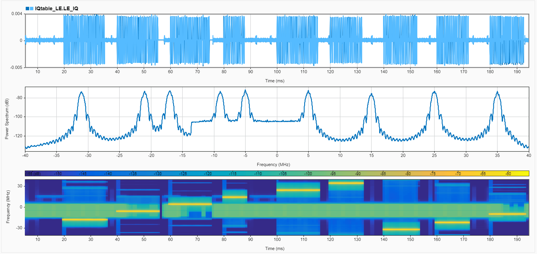
The traffic viewer visualization summarizes protocol-level behavior, while the Signal Analyzer output shows the physical layer (PHY) waveform received at the Peripheral node. When you observe them together, you see see how Bluetooth LE and WLAN transmissions in the traffic timeline correspond to the IQ samples captured by the wireless IQ logger. The IQ logger logs the received PHY waveform at the antenna of the node. The logger does not directly capture the internal waveform of the transmitter. The captured IQ samples represent the combined signal that reaches the receiver, including Bluetooth LE and WLAN packets, noise, and channel effects.

In the traffic viewer, the Central node transmits short LE packets at regular intervals, and the Peripheral node receives these packets as green Reception Success segments. The WLAN AP node and STA node exchange larger frames that appear as longer, continuous transmission periods because WLAN operates at a higher data rate and sends aggregated MAC frames. The Signal Analyzer time-domain plot shows the same behavior at the IQ waveform level. Each LE reception event in the traffic viewer corresponds to a short pulse in the time-domain waveform. The Bluetooth LE packets are narrow and periodic, so they appear as short bursts separated by idle gaps.

The power spectrum view provides a frequency-domain perspective. The Bluetooth LE transmissions appear as narrowband peaks because it occupies only a small portion of the 2.4 GHz band on each hop. WLAN traffic activity appears as a wider spectral region that reflects the Wi-Fi channel bandwidth. When LE packets are received during periods of WLAN transmission, the spectrum view shows the overlap between the LE hop frequency and the active WLAN channel.

Observe that the spectrogram plot and the channel occupancy plot of the traffic viewer provide the closest visual match. The Bluetooth LE frequency hopping appears as short, narrow regions that move across frequencies over time. WLAN transmissions appear as continuous horizontal bands centered around the WLAN operating frequency. When you compare the spectrogram with the channel occupancy plot, the LE hop positions and WLAN channel usage align directly. This alignment shows how the Peripheral node experiences the shared channel and how coexistence affects the received waveform.

This figure shows the time-domain waveform, power spectrum, and spectrogram of the IQ samples captured in the IQTable_WLAN timetable.

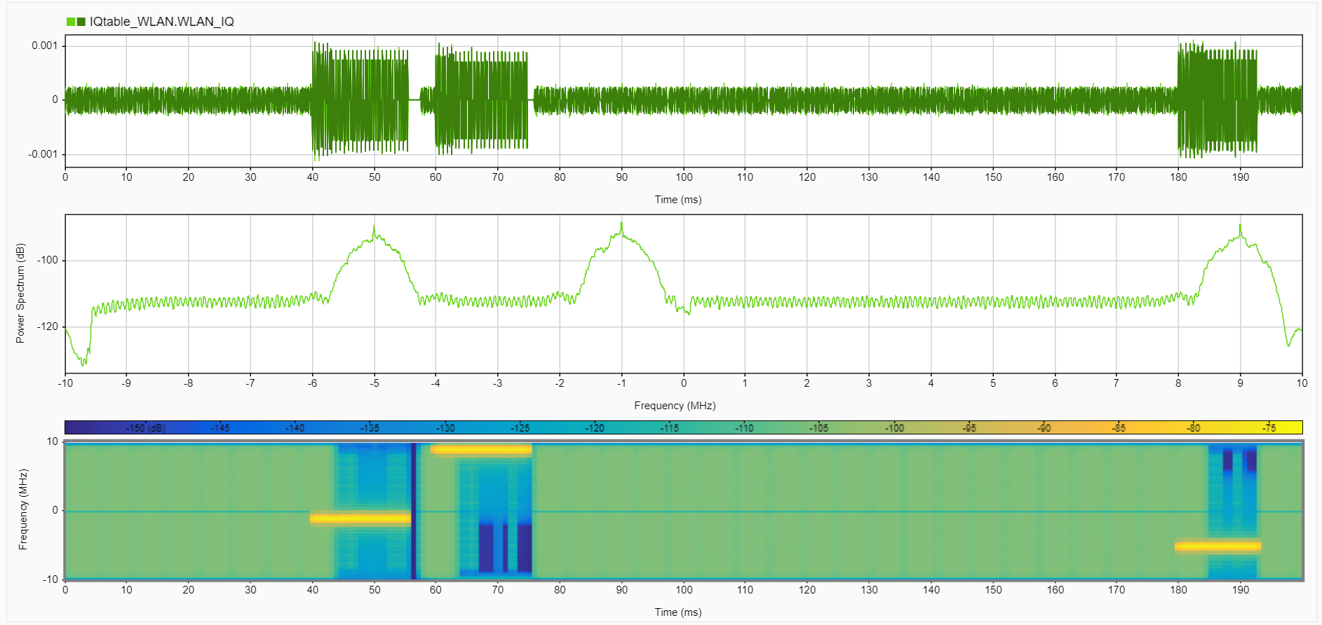
The WLAN IQ data captured at the STA node provides the PHY view of what the STA received during the simulation. The received power depends on the transmit power, distance, and pathloss. Because the Central node might be closer to the STA node than the AP node, the LE packets can appear stronger than WLAN packets in the IQ display. You can equalize signals by using similar transmit power settings or by placing the transmitters at comparable distances.

The WLAN IQ capture includes Bluetooth LE signals as well, and the Bluetooth LE IQ capture includes WLAN signals. The receiver processes whatever arrives at its antenna, and the IQ logger logs that combined signal for analysis.

In the time-domain display, you can see the extended periods of high-energy signal activity whenever the AP node transmits aggregated data frames to the STA node. These periods correspond directly to the long WLAN transmission intervals shown in the traffic viewer. Between these intervals, the waveform amplitude decreases significantly, matching the periods where the AP node is idle or the STA node is receiving only noise.

The power spectrum view shows power concentrated over a wideband region consistent with the WLAN channel bandwidth. The default spectrum view shows the power across the entire capture interval, so it reflects average spectral occupancy. To inspect the bandwidth and spectral shape of a single LE or WLAN packet, select the time of only that packet region and recompute the spectrum. This new view reveals the actual modulation bandwidth and power profile of the individual transmission. Peaks near the center frequency represent the active WLAN carrier and surrounding subcarriers. This wideband spectral shape matches the WLAN channel occupied by the AP node and STA node in the channel occupancy plot of the traffic viewer. When the traffic viewer displays a long, yellow bar indicating WLAN activity around the configured channel frequency, the power spectrum plot shows corresponding high energy across that same bandwidth.

In the spectrogram, WLAN transmissions appear as continuous regions of elevated power at the WLAN channel frequency, extending horizontally over time. These high-power regions align precisely with the long yellow occupancy blocks in the traffic viewer. The transitions between active and idle periods also match. Whenever the traffic viewer shows the AP node entering a transmission state, the spectrogram displays a corresponding section of high energy at the STA node.

By visualizing and analyzing the time-domain waveform, power spectrum, and spectrogram plots alongside the traffic viewer output, you can obtain a clear mapping from protocol-level traffic events to the received PHY waveform.

References

[1] Bluetooth^® Technology Website. “Bluetooth Technology Website | The Official Website of Bluetooth Technology.” Accessed December 22, 2025. https://www.bluetooth.com/.

[2] Bluetooth Special Interest Group (SIG). "Bluetooth Core Specification." v6.1. https://www.bluetooth.com/specifications/specs/core-specification-6-1/.