Analyze Link Viability of Cellular Network with Mobile UEs Using Ray Tracing
This example shows how to create a scenario for analyzing a network modeling one sectorized base station (three gNBs), and five UEs distributed across the three sectors.
Three UEs are in motion.
Two UEs are stationary.
Some of the UEs have line-of-sight access to the base station and some do not.
In this example, you estimate the received signal strength (RSS) at each UE over time as they move along their respective trajectories. To determine the viability of this configuration, you compare the signal strength to receiver sensitivity levels. Specifically, you determine if the various links operate successfully in the environment.
Scenario Description
The scenario is based on a map of the same part of Boston used in the Mobility Modeling with Ray Tracing Channel example, expanding the scene to accommodate more nodes. First load a map showing buildings in a portion of downtown Boston and define a trajectory by setting a couple of waypoints on a major road and creating a straight line path between the waypoints. The initial control points were obtained by right-clicking the map in Site Viewer to get latitude and longitude coordinates for the start point, stop point, and any turn points. Those coordinates define the mobile paths in the simulation. You create the view in Site Viewer by using a siteviewer object.
Create a Site Viewer instance so that building data from Open Street Maps can be added to the default geographic data:
myscenarioFile = "bostonNetworkMap.osm";
mysv = siteviewer(Buildings=myscenarioFile)
mysv =
siteviewer with properties:
Name: 'Site Viewer'
Position: [560 240 800 600]
CoordinateSystem: "geographic"
Basemap: 'satellite'
Terrain: 'gmted2010'
Buildings: 'bostonNetworkMap.osm'
Materials: [7×2 table]
The scenario includes five UEs in a Boston, Massachusetts, USA scene.
1. A person in a car driving on a city street
carSpeed = 50; % km/hr
carControlPts = ...
    [42.341482 -71.086650; 42.341102 -71.087238; 42.339903 -71.090416];
[carPts, carDist] = defineTrajectory(carControlPts,"Car");
2. A person riding a bicycle
bikeSpeed = 20; % km/hr
bikeControlPts = ...
    [42.342056, -71.095497; 42.341459, -71.095012; 42.340887, -71.093438];
[bikePts, bikeDist] = defineTrajectory(bikeControlPts,"Bike");
3. A person walking
walkerSpeed = 5; % km/hr
walkerControlPts = [42.343971,-71.084927; 42.345319,-71.083341];
[walkerPts, walkerDist] = defineTrajectory(walkerControlPts,"Walker");
4. A person sitting on a park bench in the Back Bay Fens (stationary)
sittingPersonFensPos = [42.342174,-71.093978]; % Sitting on bench by World War II Vets Memorial
sitter1Pts = defineTrajectory(sittingPersonFensPos,"ParkBenchSitter");
5. A person sitting in the bleachers at Fenway Park (stationary)
sittingPersonFenwayPos = [42.347081,-71.097579]; % In a green monster seat
sitter2Pts = defineTrajectory(sittingPersonFenwayPos,"RedSoxFan");
Base Station Placement
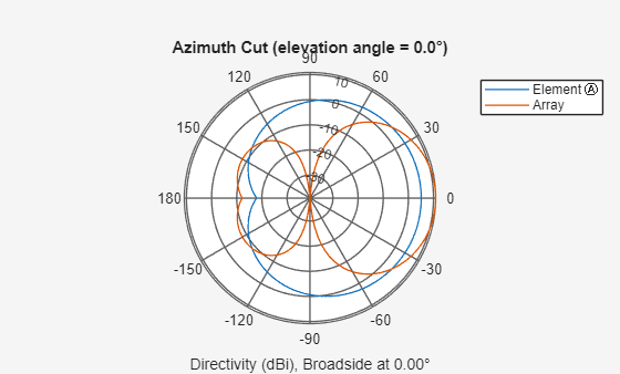
Place the base station (BS) near the geographical center of the scene. Then visualize the individual element spatial pattern as well as the array pattern, taking into account all elements.
% Set center frequency and sample rate and other shared parameters
fc = 2.6e9; % Typical for cellular systems
c = physconst("LightSpeed");
lambda = c/fc;
txHeight = 20;
totTransPwr = 10; % Watts for txsite
% For siteviewer
gNBelement1 = ...
    phased.NRAntennaElement(PolarizationAngle = -45,Beamwidth=130);
gNBelement2 = ...
    phased.NRAntennaElement(PolarizationAngle =  45,Beamwidth=130);
bsArray = phased.NRRectangularPanelArray(Size=[2 2 1 1], ...
    ElementSet={gNBelement1, gNBelement2}, ...
    Spacing= lambda * [.5 .5 1 1]);
% Visualize antenna pattern for a single element and for the array
hold off; pattern(gNBelement1, fc, -180:180, 0)
hold on; pattern(bsArray, fc, -180:180, 0)
legend("Element", "Array")
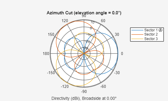
panel = phased.URA('Element',gNBelement1,'Size',[2 2], ...
    'ElementSpacing',[0.5 0.5]*lambda);
% Visualize the three sectorized array patterns simultaneously In reality,
% sectorized means three co-located antennas with different orientation.
% Subarrays are used just to get composite pattern plot. Use URA with
% ReplicatedSubarray to see sectorized pattern. (Not supported by
% NRRectangularPanelArray.)
ant = phased.ReplicatedSubarray('Subarray',panel,'Layout','Custom', ...
    'SubarrayPosition',[1 -0.5 -0.5;0 sqrt(3)/2 -sqrt(3)/2;0 0 0]*lambda, ...
    'SubarrayNormal',[0 120 -120;0 0 0]);
figure
pattern(ant,fc,-180:180,0,'Weights',[1;0;0]);
hold on;
pattern(ant,fc,-180:180,0,'Weights',[0;1;0]);
pattern(ant,fc,-180:180,0,'Weights',[0;0;1]);
legend("Sector 1", "Sector 2", "Sector 3")
hold off
txPos = [42.344423,-71.091060];
tx = txsite(Name="5G", ...
    Latitude=txPos(1),Longitude=txPos(2), ...
    Antenna=bsArray,AntennaHeight=txHeight,TransmitterFrequency=fc, ...
    TransmitterPower=totTransPwr);
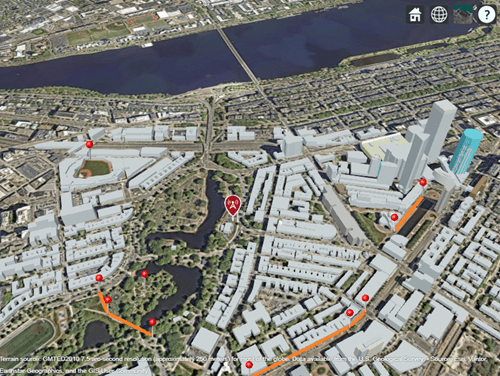
Now show all trajectories in one view that includes the stationary BS.
show([walkerPts carPts bikePts sitter1Pts sitter2Pts])
show(tx)
Compute Waypoints for UEs
Compute waypoints for the UEs along their respective paths where the analysis happens. Use the dspace parameter to set how often along a trajectory the ray tracing operation repeats. This example computes RSS only, but you can get other computations such as channel estimates at each waypoint. Because the UEs are traveling at different ground speeds, the times of these ray tracings will be different for each UE and each trajectory. Therefore, record the times of the ray tracings for each UE so that you can compare computations across UEs.
The fastest moving UE in this example is the car at carSpeed km/hr:
carSpeed
carSpeed =
50
% Specify receive array
UEelement1 = createUEAntennaElement(-45, fc);
UEelement2 = createUEAntennaElement(45, fc);
ueArray = phased.NRRectangularPanelArray(Size=[1 1 1 1], ...
    ElementSet={UEelement1, UEelement2}, Spacing=lambda * [.5 .5 1 1]);
Use the computeWaypoints local function to define the route by starting at one end and then moving on a straight line between the control points specified above, estimating the channel all along the trajectory with spatial granularity defined by dspace. The code has no checking to make sure that this path is viable in the real world, so manually verify that no points are defined in illogical locations, such as inside a building or on a lamp post. Under the assumption that the straight line path is valid, you can programmatically determine the intermediate waypoints from the initial manually defined stop, start, and turn waypoints.
Compute waypoints for each mobile UE along its path.
rxSensitivity = -100; % dBm
ueHeight = 1.5; % meters
ueFenwayHeight = 10;
dspace = 5;
% Car
[rxsCar, carDist] = computeWaypoints( ...
    carPts,dspace,ueArray,false,fc,ueHeight,rxSensitivity);
carTimes = computeWayptTimes(carDist,dspace,carSpeed);
carTimes = carTimes(1:length(rxsCar)); % Make sure time vector has same length as way points
% Bike
[rxsBike, bikeDist] = computeWaypoints( ...
    bikePts,dspace,ueArray,false,fc,ueHeight,rxSensitivity);
bikeTimes = computeWayptTimes(bikeDist,dspace,bikeSpeed);
bikeTimes = bikeTimes(1:length(rxsBike));
% Walker
[rxsWalker, walkerDist] = computeWaypoints( ...
    walkerPts,dspace,ueArray,false,fc,ueHeight,rxSensitivity);
walkerTimes = computeWayptTimes(walkerDist,dspace,walkerSpeed);
walkerTimes = walkerTimes(1:length(rxsWalker));
% No waypoint computation for stationary UEs.
rxSitter1 = rxsite(Name="ParkBenchSitter", ...
    Latitude=sittingPersonFensPos(1), ...
    Longitude=sittingPersonFensPos(2),Antenna=ueArray, ...
    AntennaHeight=ueHeight,ReceiverSensitivity=rxSensitivity);
sitter1Times = [0;Inf];
rxSitter2 = rxsite(Name="RedSoxFan",...
    Latitude=sittingPersonFenwayPos(1), ...
    Longitude=sittingPersonFenwayPos(2),Antenna=ueArray, ...
    AntennaHeight=ueFenwayHeight,ReceiverSensitivity=rxSensitivity);
sitter2Times = [0; Inf];
show([rxsCar rxsBike rxsWalker],ShowAntennaHeight=false, ...
    Icon="OrangeDot.png",IconSize=[5 5])
show([walkerPts carPts bikePts sitter1Pts sitter2Pts])
Examine signal strength at the UEs with the trajectory specified and locations determined for the fixed BS and mobile UE. Since this BS is sectorized, you must add the sectorization information for each BS to see which UEs are served by which sectors.
Configure Sectorized Base Station
Configure the BS antenna array as a single four-element rectangular panel array, which attaches to each of three identical, co-located base stations that are rotated relative to each by 120 degrees in azimuth.
tx1 = txsite(Name="5G Sector 1", ...
    Latitude=txPos(1),Longitude=txPos(2), ...
    Antenna=bsArray,TransmitterFrequency=fc, ...
    AntennaAngle=0,AntennaHeight = txHeight, ...
    TransmitterPower=totTransPwr);
tx2 = txsite(Name="5G Sector 2", ...
    Latitude=txPos(1),Longitude=txPos(2), ...
    Antenna=bsArray,TransmitterFrequency=fc, ...
    AntennaAngle=120,AntennaHeight = txHeight, ...
    TransmitterPower=totTransPwr);
tx3 = txsite(Name="5G Sector 3", ...
    Latitude=txPos(1),Longitude=txPos(2), ...
    Antenna=bsArray,TransmitterFrequency=fc, ...
    AntennaAngle=240,AntennaHeight = txHeight, ...
    TransmitterPower=totTransPwr);

pattern(tx1); pattern(tx2); pattern(tx3)
Compute Received Signal Strength
Compute the RSS along trajectories and assign sectors to serve each UE. Check the configured network to make sure each UE receives relevant signals with a sufficient power level for the link to close. Relative to the BS, each of the UEs is at a different angle and distance away. Additionally, some of the UEs are moving. The antenna for each sector has no back baffle, so each sector receives signals across 360 degrees of azimuth. In this section, you examine the downlink received signal levels at each UE from each sector of the BS. In the next section, you assign UEs to sectors and determine whether any hand-offs are required.
This example uses the sigstrength function to compare the signal strength along the each trajectory from each gNB (sector) for a ray tracing propagation model. Regarding antenna pointing direction, this example does not apply steering at the gNBs or at the UEs. The assumption is that each sector receives all signals in that sector well, without any additional steering. In addition, the antennas on the UEs are approximately omnidirectional for this example, so no steering is required for the UE antennas either.
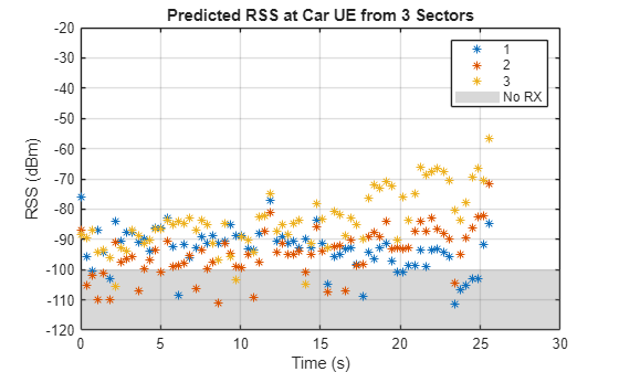
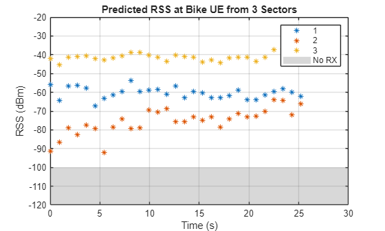
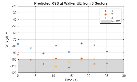
For each UE, a plot shows the RSS versus time. For each plot, the region below the sensitivity level of the receiver is marked as a gray region. For successful reception, the RSS must remain above the gray region. This visualization helps to make it clear which sectors map best to a given UE.
% Set propagation models for use in sigstrength computations below.
numreflecs = 3;
numdifracs = 1;
maxrelpathloss = 30; % Any path more than 20db below strongest is dropped
rtpropmdl = propagationModel("raytracing", ...
    MaxNumReflections=numreflecs, ...
    MaxNumDiffractions=numdifracs, ...
    MaxRelativePathLoss=maxrelpathloss,UseGPU="auto");
Warning: Support for GPU devices with compute capability 6.1 will be removed in a future MATLAB release. For more information on GPU support, see <a href="matlab:web('http://www.mathworks.com/help/parallel-computing/gpu-computing-requirements.html','-browser')">GPU Computing Requirements</a>.
% Show signal strength at each UE from each sectorized gNB
alltxs = [tx1, tx2, tx3];
alltimepts = sigstrength(rxsCar,alltxs,rtpropmdl);
figure;
plot(carTimes,alltimepts.',"*");
legend("1","2","3")
yr=yregion(-Inf,rxSensitivity);
yr.DisplayName="No RX";
grid on
axis([0 30 -120 -20])
title("Predicted RSS at Car UE from 3 Sectors")
ylabel("RSS (dBm)");
xlabel("Time (s)")
bikeTimes = bikeTimes(bikeTimes<=carTimes(end));
alltimepts = sigstrength(rxsBike(1:length(bikeTimes)),alltxs,rtpropmdl);
figure; plot(bikeTimes, alltimepts.', "*"); legend("1", "2", "3")
yr = yregion(-Inf,rxSensitivity);
yr.DisplayName="No RX";
grid on
xlim([0.0 30.0]);
ylim([-120 -20])
title("Predicted RSS at Bike UE from 3 Sectors")
ylabel("RSS (dBm)");
xlabel("Time (s)")
walkerTimes = walkerTimes(walkerTimes<=carTimes(end));
alltimepts = sigstrength(rxsWalker(1:length(walkerTimes)),alltxs,rtpropmdl);
figure; plot(walkerTimes,alltimepts.',"*");
legend("1","2","3")
yr = yregion(-Inf,rxSensitivity);
yr.DisplayName="No RX";
grid on
xlim([0.0 30.0]);
ylim([-120 -20])
title("Predicted RSS at Walker UE from 3 Sectors")
ylabel("RSS (dBm)");
xlabel("Time (s)")
xlim([0.0 30.0]); ylim([-120 -20])
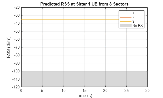
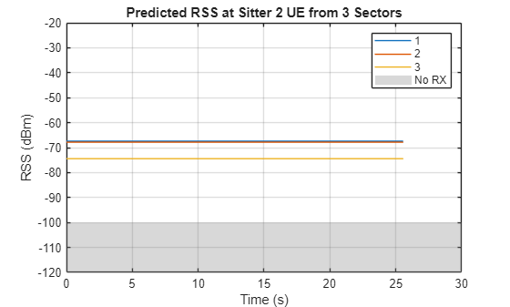
The two stationary UEs will have constant RSS during the observation interval.
alltimepts = sigstrength(rxSitter1,alltxs,rtpropmdl);
figure;
plot(carTimes,ones(size(carTimes.'))*alltimepts.');
legend("1","2","3")
yr=yregion(-Inf, rxSensitivity);
yr.DisplayName="No RX";
grid on
axis([0 30 -120 -20])
title("Predicted RSS at Sitter 1 UE from 3 Sectors")
ylabel("RSS (dBm)");
xlabel("Time (s)")
alltimepts = sigstrength(rxSitter2,alltxs, rtpropmdl);
figure;
plot(carTimes,ones(size(carTimes.'))*alltimepts.');
legend("1","2","3")
yr = yregion(-Inf,rxSensitivity);
yr.DisplayName="No RX";
grid on
axis([0 30 -120 -20])
title("Predicted RSS at Sitter 2 UE from 3 Sectors")
ylabel("RSS (dBm)");
xlabel("Time (s)")
Analyze Scene Geometry
Analyze the scenario to determine the ideal sector for each UE over their entire trajectories. In the previous section, you looked at RSS to determine which BS sector best serves each UE. In this section, you analyze the geometry in the scene to see how the layout and obstacles influences sector assignment. Then you, compare the geometric analysis results with the RSS results.
The walker UE appears to be approximately due east from the BS and the first sectorized BS points due east. You can verify these locations by using the angle() function:
walkerInitAngleFromBase = angle(tx,rxsWalker(1))
walkerInitAngleFromBase =
-5.6715
Since the walker is moving, compare the initial and final trajectory points to determine the change in angle.
walkerTotalAngle = angle(tx,rxsWalker(end)) - angle(tx,rxsWalker(1))
walkerTotalAngle =
14.3342
The angle change is small enough to be confident that no hand-off between sectors occur for the walker UE over the duration of this trajectory. This result aligns with the RSS results in the previous section. The RSS from sector 1 is the strongest for the walker UE.
Apply similar analysis to the other UEs to determine sector assignments and determine if any hand-offs are required.
For the car UE:
carInitAngleFromBase= angle(tx,rxsCar(1))
carInitAngleFromBase =
-41.9529
carTotalAngle = angle(tx,rxsCar(end)) - angle(tx,rxsCar(1))
carTotalAngle =
-41.7627
The dividing line between sector 1 and sector 3 occurs at –60 degrees. The car starts in sector 1 but moves to sector 3 as it moves along its trajectory. However, the car never has line-of-sight access to the BS, so the signal strength analysis above does not always clearly indicate a preferred sector. The car moves across the –60 degree sector boundary at about 11 seconds along the path. From that point forward, a clear preference toward sector 3 is indicated in the RSS plot from the previous section.
For the biker UE:
bikeInitAngleFromBase= angle(tx,rxsBike(1))
bikeInitAngleFromBase =
-144.2812
bikeTotalAngle = angle(tx,rxsBike(end)) - angle(tx,rxsBike(1))
bikeTotalAngle =
26.9036
The bike is in sector 3 and remains there for its entire trajectory.
The two sitting UEs do not move, so their analysis is easier:
sitter1AngleFromBase = angle(tx,rxSitter1)
sitter1AngleFromBase =
-133.9068
sitter2AngleFromBase = angle(tx,rxSitter2)
sitter2AngleFromBase =
151.2028
Sitter 1 is in sector 3 and sitter 2 is in sector 2. No hand-offs are required because these UEs are stationary for the duration of the simulation.
For the biker and the two sitters, the geometric analysis matches well with the RSS analysis.
Check Line-of-Sight
Check if and when the various UEs have line-of-sight access to their assigned BS.
% Each trajectory in this scenario either always has line-of-sight
% or never has it.
mylosCar = los(tx1,rxsCar);
if ~any(mylosCar), disp("No LOS access on car trajectory."), end
No LOS access on car trajectory.
mylosBike = los(tx3,rxsBike);
if all(mylosBike), disp("Entire bike trajectory has LOS access."), end
Entire bike trajectory has LOS access.
mylosWalker = los(tx1,rxsWalker);
if ~any(mylosWalker), disp("No LOS access on walker trajectory."), end
No LOS access on walker trajectory.
mylosSitter1 = los(tx3,rxSitter1);
if all(mylosSitter1), disp("Sitter 1 has LOS access."), end
Sitter 1 has LOS access.
mylosSitter2 = los(tx2,rxSitter2);
if ~any(mylosSitter2), disp("No LOS access for sitter 2."), end
No LOS access for sitter 2.
Further Exploration
Once the setup of this scenario is viable, then a second more thorough network simulation can be attempted.
You can run the helper
computeAndSaveChannelsAndTrajectoriesscript to storecomm.RayTracingChannelfor each UE along their respective trajectories along with the coordinates of those trajectories.You can use the channel models and trajectory definitions in a network level simulation to analyze throughput and other such metrics for this same scenario.
Local Functions
The example uses these local functions.
function [wayptRxsites, totalDist] = computeWaypoints(controlPts,spacing,ueArray, useTx, fc, myHeight, rxSensitivity)
% Compute waypoints between control points on the map.
arguments
    controlPts (1,:)
    spacing (1,1) {mustBeNumeric}=5
    ueArray (1,1) = phased.IsotropicAntennaElement;
    useTx (1,1) logical=false
    fc (1,1) {mustBeNumeric} = 2e9
    myHeight (1,1) = 0
    rxSensitivity (1,1) double=-100
end
theDist = 0;
myDist = 0;
idx = 0;
offset = 0;
if useTx
    rxs = txsite.empty;
else
    rxs = rxsite.empty;
end
for sgmntIdx = 1 : numel(controlPts)-1 % Road segment
    theDist = theDist + ...
        distance(controlPts(sgmntIdx),controlPts(sgmntIdx+1));
    az = angle(controlPts(sgmntIdx),controlPts(sgmntIdx+1));
    [lat,lon] = location(controlPts(sgmntIdx),offset,az);
    % Set next point on this segment
    idx = idx + 1;
    locname = sprintf(" P%d",idx);
    if useTx
        rxs(idx) = txsite(Name=locname,...
            Latitude=lat, Longitude=lon, Antenna=ueArray, ...
            AntennaHeight=myHeight, TransmitterFrequency=fc);
    else
        rxs(idx) = rxsite(Name=locname,...
            Latitude=lat, Longitude=lon, Antenna=ueArray, ...
            AntennaHeight=myHeight, ReceiverSensitivity=rxSensitivity);
    end
    myDist = myDist + spacing;
    while myDist+offset < theDist
        % Next point on current segment
        [lat,lon] = location(rxs(idx),spacing,az);
        idx = idx+1;
        % Set next point on this segment
        locname = sprintf("P%d",idx);
        if useTx % Allow for mobile TX instead of RX
            rxs(idx) = txsite(Name=locname, ...
                Latitude=lat, Longitude=lon, Antenna=ueArray, ...
                AntennaHeight=myHeight, ...
                TransmitterFrequency=fc);
        else
            rxs(idx) = rxsite(Name=locname, ...
                Latitude=lat, Longitude=lon, Antenna=ueArray, ...
                AntennaHeight=myHeight);
        end
        myDist = myDist + spacing;
    end
    offset = myDist - theDist;
end
wayptRxsites = rxs;
totalDist = theDist;
end
%%
function myTimes = computeWayptTimes(totalDist, deltaDist, myspeed)
% Compute times from waypoint to waypoint.
myspeedMetersPerSec = myspeed * 1000 / 3600;
deltaT    = deltaDist / myspeedMetersPerSec;
totalTime = totalDist / myspeedMetersPerSec;
myTimes = 0:deltaT:totalTime;
end
%%
function [controlPts, totDist] = defineTrajectory(controlPoints,myname,useTxSite)
% Mark begin, end and bends to define a trajectory. A pin is dropped at
% each control point to define the path of the trajectory, which consists
% of straight line segments from one control point to the next.
arguments
    controlPoints (:,2)
    myname (1,1) string="traj"
    useTxSite (1,1) logical=false
end
%
% Format of controlPoints:
%   Nx2. Each row is Lat, Long
%
if useTxSite
    controlPts = txsite("geographic", ...
        Latitude=controlPoints(:,1),...
        Longitude=controlPoints(:,2));
else
    controlPts = rxsite("geographic", ...
        Latitude=controlPoints(:,1),...
        Longitude=controlPoints(:,2));
end
show(controlPts,ShowAntennaHeight=false, ...
    Icon="pin.png",...
    IconSize=[12 30])
numCtrlPts = length(controlPts);
totDist = 0;
for i=1:numCtrlPts-1
    totDist = totDist + distance(controlPts(i),controlPts(i+1));
end
end
%%
function ueAntennaElement = createUEAntennaElement(polAngleDeg,fc)
% Create a custom antenna element using a short dipole element as a
% reference. POLANGLEDEG is the polarization angle in degrees relative to
% the z axes of the reference short dipole element. FC is the frequency
% used to calculate the antenna response.

% Compute polarization direction vector
polVector = [0; sind(polAngleDeg); cosd(polAngleDeg)]; % y–z plane rotation

% Create reference short dipole antenna element
shortDipole = phased.ShortDipoleAntennaElement(AxisDirection='Custom',CustomAxisDirection=polVector);

% Define angles
azAngles = -180:180;  % Azimuth angles
elAngles = -90:90;    % Elevation angles

% Extract H and V patterns in magnitude and phase
patHmag = zeros(numel(elAngles),numel(azAngles));
patVmag = patHmag;
patHphase = patHmag;
patVphase = patHmag;

for m = 1:numel(elAngles)
    pat = step(shortDipole,fc,[azAngles;elAngles(m)*ones(1,numel(azAngles))]);

    patHmag(m,:) = mag2db(abs(pat.H)); % Store horizontal pattern magnitude
    patVmag(m,:) = mag2db(abs(pat.V)); % Store vertical pattern magnitude
    patHphase(m,:) = rad2deg(angle(pat.H));        % Store horizontal pattern phase
    patVphase(m,:) = rad2deg(angle(pat.V));        % Store vertical pattern phase
end

% Initialize the custom antenna element with polarization applied
ueAntennaElement = phased.CustomAntennaElement(PatternCoordinateSystem='az-el',...
    AzimuthAngles=azAngles,ElevationAngles=elAngles,...
    SpecifyPolarizationPattern=true,...
    HorizontalMagnitudePattern=patHmag,HorizontalPhasePattern=patHphase,...
    VerticalMagnitudePattern=patVmag,VerticalPhasePattern=patVphase);

end
See Also
Objects
comm.RayTracingChannel|phased.NRRectangularPanelArray(Phased Array System Toolbox) |propagationModel|raytrace