Reducing Model Order

Model Order Reduction Commands

You can derive reduced-order SISO and MIMO models with the commands shown in the following table.

Model Order Reduction Commands
`hsvd`	Compute Hankel singular values of LTI model
`balred`	Reduced-order model approximation
`minreal`	Minimal realization (pole/zero cancellation)
`balreal`	Compute input/output balanced realization
`modred`	State deletion in I/O balanced realization
`sminreal`	Structurally minimal realization

Techniques for Reducing Model Order

To reduce the order of a model, you can perform any of the following actions:

Eliminate states that are structurally disconnected from the inputs or outputs using sminreal.
Eliminating structurally disconnected states is a good first step in model reduction because the process is cheap and does not involve any numerical computation.
Compute a low-order approximation of your model using balred.
Eliminate canceling pole/zero pairs using minreal.

Example: Gasifier Model

This example presents a model of a gasifier, a device that converts solid materials into gases. The original model is nonlinear.

Loading the Model

To load a linearized version of the model, type

load ltiexamples

at the MATLAB^® prompt; the gasifier example is stored in the variable named gasf. If you type

size(gasf)

you get in return

State-space model with 4 outputs, 6 inputs, and 25 states.

SISO Model Order Reduction

You can reduce the order of a single I/O pair to understand how the model reduction tools work before attempting to reduce the full MIMO model as described in MIMO Model Order Reduction.

This example focuses on a single input/output pair of the gasifier, input 5 to output 3.

sys35 = gasf(3,5);

Before attempting model order reduction, inspect the pole and zero locations by typing

pzmap(sys35)

Zoom in near the origin on the resulting plot using the zoom feature or by typing

axis([-0.2 0.05 -0.2 0.2])

The following figure shows the results.

Pole-Zero Map of the Gasifier Model (Zoomed In)

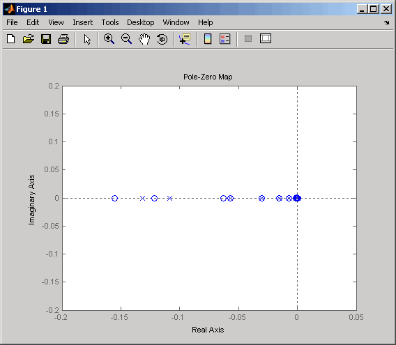
Because the model displays near pole-zero cancellations, it is a good candidate for model reduction.

To find a low-order reduction of this SISO model, perform the following steps:

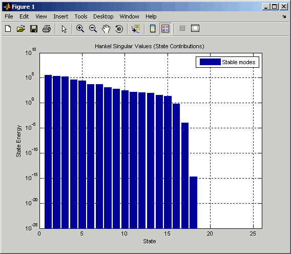
Select an appropriate order for your reduced system by examining the relative amount of energy per state using a Hankel singular value (HSV) plot. Type the command
```
hsvd(sys35)
```
to create the HSV plot.
Changing to log scale using the right-click menu results in the following plot.

Small Hankel singular values indicate that the associated states contribute little to the I/O behavior. This plot shows that discarding the last 10 states (associated with the 10 smallest Hankel singular values) has little impact on the approximation error.
To remove the last 10 states and create a 15th order approximation, type
```
rsys35 = balred(sys35,15);
```
You can type size(rsys35) to see that your reduced system contains only 15 states.
Compare the Bode response of the full-order and reduced-order models using the bode command:
```
bode(sys35,'b',rsys35,'r--')
```
This figure shows the result.
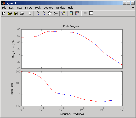
As the overlap of the curves in the figure shows, the reduced model provides a good approximation of the original system.

You can try reducing the model order further by repeating this process and removing more states. Reduce the gasf model to 5th, 10th, and 15th orders all at once by typing the following command

rsys35 = balred(sys35,[5 10 15]);

Plot a bode diagram of these three reduced systems along with the full order system by typing

bode(sys35,'b',rsys35,'r--')

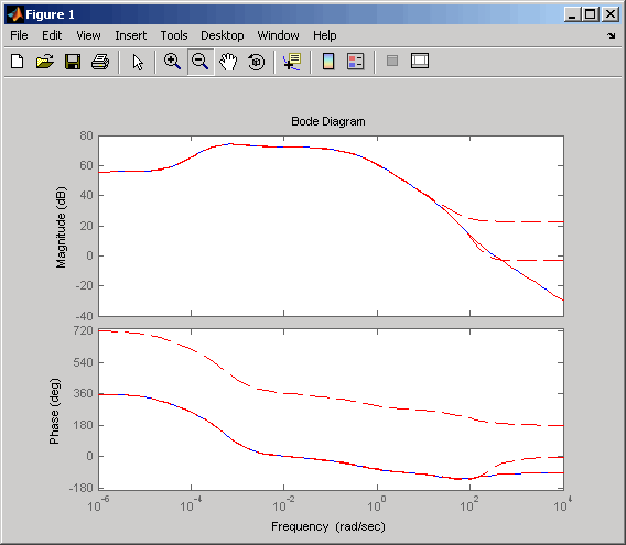
Observe how the error increases as the order decreases.

MIMO Model Order Reduction

You can approximate MIMO models using the same steps as SISO models as follows:

Select an appropriate order for your reduced system by examining the relative amount of energy per state using a Hankel singular value (HSV) plot.
Type
```
hsvd(gasf)
```
to create the HSV plot.
Discarding the last 8 states (associated with the 8 smallest Hankel singular values) should have little impact on the error in the resulting 17th order system.
To remove the last 8 states and create a 17th order MIMO system, type
```
rsys=balred(gasf,17);
```
You can type size(gasf) to see that your reduced system contains only 17 states.
To facilitate visual inspection of the approximation error, use a singular value plot rather than a MIMO Bode plot. Type
```
sigma(gasf,'b',gasf-rsys,'r')
```
to create a singular value plot comparing the original system to the reduction error.

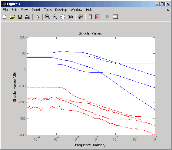
The reduction error is small compared to the original system so the reduced order model provides a good approximation of the original model.

Acknowledgment

MathWorks^® thanks ALSTOM^® Power UK for permitting use of their gasifier model for this example. This model was issued as part of the ALSTOM Benchmark Challenge on Gasifier Control. For more details see Dixon, R., (1999), "Advanced Gasifier Control," Computing & Control Engineering Journal, IEE, Vol. 10, No. 3, pp. 92–96.