networkDistributionDiscriminator
R2026bSyntax
Description
Add-On Required: This feature requires the AI Verification Library for Deep Learning Toolbox add-on.
returns a distribution discriminator using the method specified by
discriminator = networkDistributionDiscriminator(net,XID,XOOD,method)method.
You can use the discriminator to classify observations as in-distribution (ID) and out-of-distribution (OOD). OOD data refers to data that is sufficiently different from the data you use to train the network, which can cause the network to behave unexpectedly. For more information, see In-Distribution and Out-of-Distribution Data.
The networkDistributionDiscriminator function first finds
distribution confidence scores using the method you specify in method. The
function then finds a threshold that best separates the ID and OOD distribution confidence
scores. You can classify any observation with a score below the threshold as OOD. For more
information about how the function computes the threshold, see Algorithms. You can find the
threshold using a set of ID data, a set of OOD data, or both.
To determine whether new data is ID or OOD, pass discriminator as
an input to the isInNetworkDistribution function.
To find the distribution confidence scores, pass discriminator as
an input to the distributionScores function. For more information about distribution
confidence scores, see Distribution Confidence Scores.
returns a distribution discriminator using only the ID data. The
discriminator = networkDistributionDiscriminator(net,XID,[],method)Threshold property of discriminator contains the
threshold such that the discriminator attains a true positive rate greater than the value of
the TruePositiveGoal
name-value argument. For more information, see Algorithms.
returns a distribution discriminator using only the OOD data. The
discriminator = networkDistributionDiscriminator(net,[],XOOD,method)Threshold property of discriminator contains the
threshold such that the discriminator attains a false positive rate less than the value of
the FalsePositiveGoal
name-value argument. For more information, see Algorithms.
returns a discriminator with additional options specified by one or more name-value
arguments. discriminator = networkDistributionDiscriminator(___,Name=Value)
Examples
Load a pretrained classification network.
load("digitsClassificationMLPNetwork.mat");Load ID data.
XID = digitTrain4DArrayData;
Modify the ID training data to create an OOD set.
XOOD = XID*0.3 + 0.1;
Create a discriminator. The function finds the threshold that best separates the two distributions of data by maximizing the true positive rate and minimizing the false positive rate.
method = "baseline";
discriminator = networkDistributionDiscriminator(net,XID,XOOD,method)discriminator =
BaselineDistributionDiscriminator with properties:
Method: "baseline"
Network: [1×1 dlnetwork]
Threshold: 0.9743
Load a pretrained classification network.
load("digitsClassificationMLPNetwork.mat");Load ID data.
XID = digitTrain4DArrayData;
Create a discriminator using only the ID data. Set the method to "energy" with a temperature of 10. Specify the true positive goal as 0.975. To specify the true positive goal, you must specify ID data and not specify the false positive goal.
method = "energy"; discriminator = networkDistributionDiscriminator(net,XID,[],method, ... Temperature=10, ... TruePositiveGoal=0.975)
discriminator =
EnergyDistributionDiscriminator with properties:
Method: "energy"
Network: [1×1 dlnetwork]
Temperature: 10
Threshold: 23.5541
Load a pretrained classification network.
load("digitsClassificationMLPNetwork.mat");Create OOD data. In this example, the OOD data is 1000 images of random noise. Each image is 28-by-28 pixels, the same size as the input to the network.
XOOD = rand([28 28 1 1000]);
Create a discriminator. Specify the false positive goal as 0.025. To specify the false positive goal, you must specify OOD data and not specify the true positive goal.
method = "baseline"; discriminator = networkDistributionDiscriminator(net,[],XOOD,method, ... FalsePositiveGoal=0.025)
discriminator =
BaselineDistributionDiscriminator with properties:
Method: "baseline"
Network: [1×1 dlnetwork]
Threshold: 0.9998
Load a pretrained regression network.
load("digitsRegressionMLPNetwork.mat")Load ID data.
XID = digitTrain4DArrayData;
Modify the ID training data to create an OOD set.
XOOD = XID*0.3 + 0.1;
Create a discriminator. For regression tasks, set the method to "hbos". When using the HBOS method, you can specify additional options. Set the variance cutoff to 0.0001 and use the penultimate layer to compute the HBOS distribution scores.
method = "hbos"; discriminator = networkDistributionDiscriminator(net,XID,XOOD,method, ... VarianceCutoff=0.0001, ... LayerNames="relu_2")
discriminator =
HBOSDistributionDiscriminator with properties:
Method: "hbos"
Network: [1×1 dlnetwork]
LayerNames: "relu_2"
VarianceCutoff: 1.0000e-04
Threshold: -54.1241
Load a pretrained classification network.
load('digitsClassificationMLPNetwork.mat');Load ID data.
XID = digitTrain4DArrayData; numObservations = size(XID,4);
Modify the ID training data to create an OOD set.
XOOD = XID*0.3 + 0.1;
Create a discriminator. The function finds the threshold that best separates the two distributions of data.
method = "baseline";
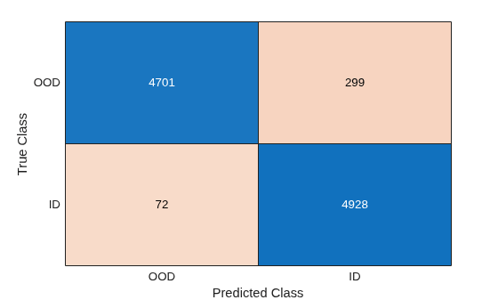
discriminator = networkDistributionDiscriminator(net,XID,XOOD,method);Test the discriminator on the ID and OOD data using the isInNetworkDistribution function. The isInNetworkDistribution function returns a logical array indicating which observations are ID and which observations are OOD.
Xdata = cat(4,XID,XOOD); trueClass = [true(numObservations,1); false(numObservations,1)]; predictedClass = isInNetworkDistribution(discriminator,Xdata);
Calculate the accuracy for the ID and OOD observations.
accuracy = sum(trueClass == predictedClass)/numel(trueClass)
accuracy = 0.9629
Create a confusion chart for the ID and OOD data.
cm = confusionchart(trueClass,predictedClass);
Display the underlying class labels.
cm.ClassLabels
ans = 2×1 logical array
0
1
Specify the row and column display labels in the same order.
displayLabels = ["OOD" "ID"]; cm.RowDisplayLabels = displayLabels; cm.ColumnDisplayLabels = displayLabels;
Use the distributionScores function to find the distribution scores for the ID and OOD data.
scores = distributionScores(discriminator,Xdata);
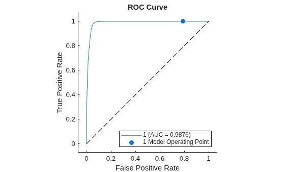
Use rocmetrics to plot a ROC curve to show how well the model is at separating the data into ID and OOD.
rocObj = rocmetrics(trueClass,scores,1); plot(rocObj)
Load a pretrained classification network.
load("digitsClassificationMLPNetwork.mat");Load the digit sample data and create an image datastore. The imageDatastore function automatically labels the images based on folder names.
digitDatasetPath = fullfile(matlabroot,'toolbox','nnet','nndemos', ... 'nndatasets','DigitDataset'); imds = imageDatastore(digitDatasetPath, ... 'IncludeSubfolders',true,'LabelSource','foldernames');
Create the minibatchqueue object.
Specify a mini-batch size of 64.
Preprocess the mini-batches using the
preprocessMiniBatchfunction, listed at the end of this example.Convert the output to a
dlarrayobject.Specify that the output data has format
"SSCB"(spatial, spatial, channel, batch).
mbq = minibatchqueue(imds, ... MiniBatchSize=64, ... MiniBatchFcn=@preprocessMiniBatch, ... OutputAsDlarray=true, ... MiniBatchFormat="SSCB");
Create a discriminator using the minibatchqueue object containing ID data. Set the method to "baseline" and the VerbosityLevel to "detailed".
method = "baseline"; discriminator = networkDistributionDiscriminator(net,mbq,[],method,VerbosityLevel="detailed");
Processing in-distribution data: Computing distribution scores... .......... .......... .......... .......... .......... (50 mini-batches) .......... .......... .......... .......... .......... (100 mini-batches) .......... .......... .......... .......... .......... (150 mini-batches) ....... (157 mini-batches) Done. Computing threshold...Done.
Mini-Batch Preprocessing Function
The preprocessMiniBatch function preprocesses the data using the following steps:
Extract the image data from the incoming cell array and concatenate the data into a numeric array.
Rescale the images to the range
[0 1].
function X = preprocessMiniBatch(dataX) X = cat(4,dataX{1:end}); X = rescale(X,InputMin=0,InputMax=1); end
Input Arguments
Neural network, specified as a dlnetwork object.
In-distribution (ID) data, specified as a formatted or unformatted dlarray object,
minibatchqueue
that has PreprocessingEnvironment set to
"serial" (default), numeric array, categorical array, datastore,
cell array, table, or []. For more information about dlarray formats,
see the fmt
input argument of dlarray.
At least one of the XID and XOOD input arguments
must be nonempty. For networks with multiple inputs, the inputs must be a minibatchqueue or
a datastore object.
For more information about ID and OOD data, see In-Distribution and Out-of-Distribution Data.
Before R2026b: If you specify the input as a minibatchqueue
object, then it must return a formatted dlarray
Out-of-distribution (OOD) data, specified as a formatted or unformatted dlarray object,
minibatchqueue
that has PreprocessingEnvironment set to
"serial" (default), numeric array, categorical array, datastore,
cell array, table, or []. For more information about dlarray formats,
see the fmt
input argument of dlarray.
At least one of the XID and XOOD input arguments
must be nonempty. For networks with multiple inputs, the inputs must be a minibatchqueue or
a datastore object.
For more information about ID and OOD data, see In-Distribution and Out-of-Distribution Data.
Before R2026b: If you specify the input as a minibatchqueue
object, then it must return an formatted dlarray
Method for computing the distribution confidence scores, specified as one of these values:
"baseline"— Use maximum softmax activations as the distribution confidence scores [1]. This method creates aBaselineDistributionDiscriminatorobject."odin"— Use rescaled softmax activations as distribution confidence scores (also known as the ODIN method) [2]. Set the scale by specifying theTemperaturename-value argument. This method creates anODINDistributionDiscriminatorobject."energy"— Use scaled, energy-based distribution confidence scores [3]. Set the scale by specifying theTemperaturename-value argument. This method creates anEnergyDistributionDiscriminatorobject."hbos"— Use histogram-based outlier scores (also known as the HBOS method) [4] as distribution confidence scores. The function computes the scores by constructing histograms for the principal component features for each layer that you specify in theLayerNamesname-value argument. Use theVarianceCutoffname-value argument to control the number of principal component features the software uses. To use this method,XIDmust be nonempty. This method creates aHBOSDistributionDiscriminatorobject."kde"— Use a smooth approximation of the underlying probability density function as distribution confidence scores. The function computes the scores using kernel density estimation (KDE) for the principal component features for each layer that you specify in theLayerNamesname-value argument. Use theVarianceCutoffname-value argument to control the number of principal component features the software uses. To use this method,XIDmust be nonempty. This method creates aKDEDistributionDiscriminatorobject. This option requires Statistics and Machine Learning Toolbox™. (since R2026a)
Tip
As the HBOS method uses histograms to estimate the underlying PDF, small changes in input values can cause abrupt jumps in the HBOS scores due to the bin boundaries. The KDE is an alternative method that can produce a smoother approximation of the underlying PDF than HBOS, but it can be more computationally expensive to create. During the execution of generated code, the accumulation of small precision errors might cause crossing of histogram bins and yield larger changes to the distribution scores. For deployment, use the KDE method to improve consistency of OOD classification decisions between development and deployed environments.
For more information about each method, see Distribution Confidence Scores.
Note
Specifying method as
"baseline", "odin", or
"energy" is valid only for single-output networks with a softmax
layer as the final layer. For example, specifying net as a
single-output classification network. You can specify method as
"hbos" or "kde" for any network.
Data Types: char | string
Name-Value Arguments
Specify optional pairs of arguments as
Name1=Value1,...,NameN=ValueN, where Name is
the argument name and Value is the corresponding value.
Name-value arguments must appear after other arguments, but the order of the
pairs does not matter.
Example: TruePositiveGoal=0.99,Temperature=10
True positive goal, specified as a scalar in the range [0, 1]. The software returns the threshold that correctly classifies at least this proportion of the ID data as ID.
Dependency
If you specify a true positive goal, then XID must
be nonempty and you cannot specify FalsePositiveGoal. If you specify a nonempty XOOD
value, then the software uses only XID to compute the
threshold.
If you do not specify the TruePositiveGoal and FalsePositiveGoal name-value arguments and provide nonempty XID and XOOD values, then the function does not use the default values and instead optimizes over the true positive rate and false positive rate to find the optimal threshold. For more information, see Algorithms.
Data Types: single | double | int8 | int16 | int32 | int64 | uint8 | uint16 | uint32 | uint64
False positive goal, specified as a scalar in the range [0, 1]. The software returns the threshold that incorrectly classifies at most this proportion of the OOD data as ID.
Dependency
If you specify a false positive goal, then XOOD must
be nonempty and you must not specify TruePositiveGoal. If you specify a nonempty XID
value, then the software uses only XOOD to compute the
threshold.
If you do not specify the TruePositiveGoal and FalsePositiveGoal name-value arguments and provide nonempty XID and XOOD values, then the function does not use the default values and instead optimizes over the true positive rate and false positive rate to find the optimal threshold. For more information, see Algorithms.
Data Types: single | double | int8 | int16 | int32 | int64 | uint8 | uint16 | uint32 | uint64
Temperature scaling for the ODIN and energy methods, specified as a positive scalar. The temperature controls the scaling of the softmax scores when the function computes the distribution confidence scores. For more information, see Distribution Confidence Scores.
Dependency
To enable this input, specify method as
"odin" or "energy".
Data Types: single | double | int8 | int16 | int32 | int64 | uint8 | uint16 | uint32 | uint64
Layer names for the HBOS or KDE method, specified as a string scalar, character
vector, string array, or cell array of character vectors. The default value is the
first layer specified in the OutputNames property of net.
The software computes the distribution confidence scores using the principal components from all of the specified layers. For more information, see Density-Based Methods.
Note
To create a discriminator, the software must first compute the principal component features for each layer. Computing the principal components can be slow for layers with a large output size and can cause you to run out of memory. If you run out of memory, try specifying layers with a smaller output size. For more information, see Density-Based Methods.
Dependency
To enable this input, specify method as
"hbos" or "kde".
Data Types: char | string | cell
Variance cutoff for the HBOS or KDE method, specified as a scalar in the range [0, 1].
The variance cutoff controls the number of principal component features that the software
uses to compute the distribution confidence scores. Using a greater number of features takes
more computation time. The closer the VarianceCutoff value is to
1, the fewer principal components the software uses to compute the
scores. For more information, see Density-Based Methods.
Dependency
To enable this input, specify method as
"hbos" or "kde".
Data Types: single | double | int8 | int16 | int32 | int64 | uint8 | uint16 | uint32 | uint64
Verbosity level of the Command Window output, specified as one of these values:
"off"— Do not display progress information."summary"— Display a summary of the progress information."detailed"— Display detailed information about the progress. This option prints the mini-batch progress.
Since R2026b
Size of mini-batches to use for prediction, specified as a positive integer. Larger mini-batch sizes require more memory, but can lead to faster predictions.
To specify padding options, use the SequenceLength name-value
argument.
Note
If you specify the input data as a
minibatchqueue object, then the
networkDistributionDiscriminator
function uses the mini-batch size specified by this argument and not the
MiniBatchSize property of the minibatchqueue
object. (since R2026b)
Data Types: single | double | int8 | int16 | int32 | int64 | uint8 | uint16 | uint32 | uint64
Since R2026b
Hardware resource, specified as one of these values:
"auto"— Use a GPU if one is available. Otherwise, use the CPU."gpu"— Use the GPU. Using a GPU requires a Parallel Computing Toolbox™ license and a supported GPU device. For information about supported devices, see GPU Computing Requirements (Parallel Computing Toolbox). If Parallel Computing Toolbox or a suitable GPU is not available, then the software returns an error."cpu"— Use the CPU.
Before R2026b: The function uses a CPU.
Since R2026b
Option to pad or truncate input sequences, specified as one of these values:
"longest"— Pad sequences in each mini-batch to have the same length as the longest sequence. This option does not discard any data, though padding can introduce noise to the neural network."shortest"— Truncate sequences in each mini-batch to have the same length as the shortest sequence. This option ensures that no padding is added, at the cost of discarding data.
To learn more about the effect of padding and truncating sequences, see Sequence Padding and Truncation.
Since R2026b
Direction of padding or truncation, specified as one of these options:
"right"— Pad or truncate sequences on the right. The sequences start at the same time step and the software truncates or adds padding to the end of each sequence."left"— Pad or truncate sequences on the left. The software truncates or adds padding to the start of each sequence so that the sequences end at the same time step.
For sequence-to-sequence neural networks (when the recurrent layers output the full sequence), any padding in the first time steps can negatively influence the predictions for the earlier time steps. Right padding helps prevent this issue by ensuring that padding doesn't appear in the initial time steps.
To learn more about the effects of padding and truncating sequences, see Sequence Padding and Truncation.
Since R2026b
Value for padding the input sequences, specified as a scalar.
Do not pad sequences with NaN, because this will cause the function
to error.
Data Types: single | double | int8 | int16 | int32 | int64 | uint8 | uint16 | uint32 | uint64
Since R2026b
Encoding of categorical inputs, specified as one of these values:
"integer"— Convert categorical inputs to their integer value. In this case, the network must have one input channel for each of the categorical inputs."one-hot"— Convert categorical inputs to one-hot encoded vectors. In this case, the network must havenumCategorieschannels for each of the categorical inputs, wherenumCategoriesis the number of categories of the corresponding categorical input.
Since R2026b
Description of the input data dimensions, specified as a string array, character vector, or cell array of character vectors.
If InputDataFormats is "auto", then the software uses the formats expected by the network input. Otherwise, the software uses the specified formats for the corresponding network input.
A deep learning data format is a string of characters, where each character describes the type of the corresponding data dimension. The characters are:
"S"— Spatial"C"— Channel"B"— Batch"T"— Time"U"— Unspecified
For example, suppose you have an array that represents a batch of sequences where the first, second, and third dimensions correspond to channels, observations, and time steps, respectively. You can describe the data as having the format "CBT" (channel, batch, time).
You can specify multiple dimensions labeled "S" or "U". You can use the labels "C", "B", and "T" at most once each. The software ignores singleton trailing "U" dimensions after the second dimension.
For a neural network with multiple inputs net, specify an array of input data formats, where InputDataFormats(i) corresponds to the input net.InputNames(i).
For more information, see Deep Learning Data Formats.
Data Types: char | string | cell
Output Arguments
Distribution discriminator, returned as a BaselineDistributionDiscriminator, ODINDistributionDiscriminator, EnergyDistributionDiscriminator, HBOSDistributionDiscriminator, or KDEDistributionDiscriminator object.
The function returns this output as a BaselineDistributionDiscriminator, ODINDistributionDiscriminator, EnergyDistributionDiscriminator, HBOSDistributionDiscriminator, or KDEDistributionDiscriminator (since R2026a) object when you specify method as
"baseline", "odin", "energy",
"hbos", or "kde" respectively.
The Threshold property of discriminator
contains the threshold for separating the ID and OOD data. To access the threshold
value, call discriminator.Threshold.
More About
In-distribution (ID) data refers to any data that you use to construct and train your model. Additionally, any data that is sufficiently similar to the training data is also said to be ID.
Out-of-distribution (OOD) data refers to data that is sufficiently different to the training data. For example, data collected in a different way, at a different time, under different conditions, or for a different task than the data on which the model was originally trained. Models can receive OOD data when you deploy them in an environment other than the one in which you train them. For example, suppose you train a model on clear X-ray images but then deploy the model on images taken with a lower-quality camera.
OOD data detection is important for assigning confidence to the predictions of a network. For more information, see OOD Data Detection.
OOD data detection is a technique for assessing whether the inputs to a network are OOD. For methods that you apply after training, you can construct a discriminator which acts as an additional output of the trained network that classifies an observation as ID or OOD.
The discriminator works by finding a distribution confidence score for an input. You can then specify a threshold. If the score is less than or equal to that threshold, then the input is OOD. Two groups of metrics for computing distribution confidence scores are softmax-based and density-based methods. Softmax-based methods use the softmax layer to compute the scores. Density-based methods use the outputs of layers that you specify to compute the scores. For more information about how to compute distribution confidence scores, see Distribution Confidence Scores.
These images show how a discriminator acts as an additional output of a trained neural network.
Example Data Discriminators
| Example of Softmax-Based Discriminator | Example of Density-Based Discriminator |
|---|---|
|
For more information, see Softmax-Based Methods. |
For more information, see Density-Based Methods. |
Distribution confidence scores are metrics for classifying data as ID or OOD. If an input has a score less than or equal to a threshold value, then you can classify that input as OOD. You can use different techniques for finding the distribution confidence scores.
ID data usually corresponds to a higher softmax output than OOD data [1]. Therefore, a method of defining distribution confidence scores is as a function of the softmax scores. These methods are called softmax-based methods. These methods only work for classification networks with a single softmax output.
Let ai(X) be the input to the softmax layer for class i. The output of the softmax layer for class i is given by this equation:
where C is the number of classes and
T is a temperature scaling. When the network predicts the class
label of X, the temperature T is set to
1.
The baseline, ODIN, and energy methods each define distribution confidence scores as functions of the softmax input.
Density-based methods compute the distribution scores by describing the underlying features learned by the network as probabilistic models. Observations falling into areas of low density correspond to OOD observations.
To model the distributions of the features, you can estimate the probability density function (PDF) for each feature using a histogram or KDE. This technique is based on the histogram-based outlier score (HBOS) method [4]. These methods use a data set of ID data, such as training data, to construct histograms or kernel density estimates representing the density distributions of the ID features. These methods have three stages:
Find the principal component features for which to compute the distribution confidence scores:
For each specified layer, find the activations using the n data set observations. Flatten the activations across all dimensions except the batch dimension.
Compute the principal components of the flattened activations matrix. Normalize the eigenvalues such that the largest eigenvalue is 1 and corresponds to the principal component that carries the greatest variance through the layer. Denote the matrix of principal components for layer l by Q(l).
The principal components are linear combinations of the activations and represent the features that the software uses to compute the distribution scores. To compute the score, the software uses only the principal components whose eigenvalues are greater than the variance cutoff value σ.
Note
The HBOS and KDE algorithms assume that the features are statistically independent. The principal component features are pairwise linearly independent but they can have nonlinear dependencies. To investigate feature dependencies, you can use functions such as
corr(Statistics and Machine Learning Toolbox). For an example showing how to investigate feature dependence, see Out-of-Distribution Data Discriminator for YOLO v4 Object Detector. If the features are not statistically independent, then the algorithm can return poor results. Using multiple layers to compute the distribution scores can increase the number of statistically dependent features.
For each of the principal component features with an eigenvalue greater than σ, construct a density estimate using either a histogram (HBOS) or KDE.
For histograms, the software adjusts the width of the bins to create bins of approximately equal area, where N is the number of observations. The software then normalizes the bins such that the largest height is 1.
For KDE, the software uses the Ramer–Douglas–Peucker algorithm to reduce the number of points. The software linearly interpolates between the remaining KDE points and then normalizes the density to sum to 1.
Find the distribution score for an observation by summing the logarithmic probabilities evaluated at the observation for each of the feature density estimates, over each layer.
Let f(l)(X) denote the output of layer l for input X. Use the principal components to project the output into a lower dimensional feature space using this equation: .
Compute the confidence score using this equation:
where N(l)(σ) is the number of principal components with an eigenvalue greater than σ in layer l, L is the number of layers, and
For the HBOS method, hk(l) is the normalized histogram height.
For the KDE method, hk(l) is the reduced KDE value.
A larger score corresponds to an observation that lies in the areas of higher density. If the density estimate evaluates to 0 for any feature, for example if the observation lies outside of the range of any of the histograms, then the confidence score is
-Inf.Note
The distribution scores depend on the properties of the data set the algorithm uses to approximate the PDF.
Algorithms
The function creates a discriminator using the trained network. The discriminator behaves as an additional output of the network and classifies an observation as ID or OOD using a threshold. For more information, see OOD Data Detection.
To compute the distribution threshold, the function first computes the distribution
confidence scores using the method that you specify in the method input
argument. For more information, see Distribution Confidence Scores. The software then finds the
threshold that best separates the scores of the ID and OOD data. To find the threshold, the
software optimizes over these values:
True positive goal — Number of ID observations that the discriminator correctly classifies as ID. To optimize for this value, the ID data
XIDmust be nonempty and you must specifyTruePositiveGoal. If you specifyTruePositiveGoalasp, then the software finds the threshold above which the proportion of ID confidence scores isp. This process is equivalent to finding the 100(1-p)-th percentile for the ID confidence scores.False positive goal — Number of OOD observations that the discriminator incorrectly classifies as ID. To optimize for this value, the OOD data
XOODmust be nonempty and you must specifyFalsePositiveGoal. If you specifyFalsePositiveGoalasp, then the software finds the threshold above which the proportion of OOD confidence scores isp. This process is equivalent to finding the 100p-th percentile for the OOD confidence scores.
If you provide ID and OOD data and do not specify TruePositiveGoal or
FalsePositiveGoal,
then the software finds the threshold that maximizes the balanced accuracy . If you provide only ID data, then the software optimizes using only
TruePositiveGoal,
whose default is 0.95. If you provide only OOD data, then the software
optimizes using only FalsePositiveGoal,
whose default is 0.05.
This figure illustrates the different thresholds that the software chooses if you optimize over both the true positive rate and false positive rate, just the true positive rate, or just the false positive rate.

References
[1] Shalev, Gal, Gabi Shalev, and Joseph Keshet. “A Baseline for Detecting Out-of-Distribution Examples in Image Captioning.” In Proceedings of the 30th ACM International Conference on Multimedia, 4175–84. Lisboa Portugal: ACM, 2022. https://doi.org/10.1145/3503161.3548340.
[2] Shiyu Liang, Yixuan Li, and R. Srikant, “Enhancing The Reliability of Out-of-distribution Image Detection in Neural Networks” arXiv:1706.02690 [cs.LG], August 30, 2020, http://arxiv.org/abs/1706.02690.
[3] Weitang Liu, Xiaoyun Wang, John D. Owens, and Yixuan Li, “Energy-based Out-of-distribution Detection” arXiv:2010.03759 [cs.LG], April 26, 2021, http://arxiv.org/abs/2010.03759.
[4] Markus Goldstein and Andreas Dengel. "Histogram-based outlier score (hbos): A fast unsupervised anomaly detection algorithm." KI-2012: poster and demo track 9 (2012).
[5] Jingkang Yang, Kaiyang Zhou, Yixuan Li, and Ziwei Liu, “Generalized Out-of-Distribution Detection: A Survey” August 3, 2022, http://arxiv.org/abs/2110.11334.
[6] Lee, Kimin, Kibok Lee, Honglak Lee, and Jinwoo Shin. “A Simple Unified Framework for Detecting Out-of-Distribution Samples and Adversarial Attacks.” arXiv, October 27, 2018. http://arxiv.org/abs/1807.03888.
Extended Capabilities
Usage notes and limitations:
To load a discriminator object for code generation, use the
coder.loadNetworkDistributionDiscriminatorfunction.Requires the MATLAB® Coder™ Interface for Deep Learning support package. If this support package is not installed, use the Add-On Explorer. To open the Add-On Explorer, go to the MATLAB® Toolstrip and click Add-Ons > Get Add-Ons.
Usage notes and limitations:
To load a discriminator object for code generation, use the
coder.loadNetworkDistributionDiscriminatorfunction.Requires the GPU Coder™ Interface for Deep Learning support package. If this support package is not installed, use the Add-On Explorer. To open the Add-On Explorer, go to the MATLAB® Toolstrip and click Add-Ons > Get Add-Ons.
The networkDistributionDiscriminator function fully supports GPU acceleration.
By default, the networkDistributionDiscriminator
function uses a GPU is one is available. You can specify the hardware that the
networkDistributionDiscriminator function uses by setting the ExecutionEnvironment argument. (since R2026b)
Before R2026b: This function runs on the GPU if either the network
learnable parameters or the input data are gpuArray objects.
For more information, see Run MATLAB Functions on a GPU (Parallel Computing Toolbox).
Version History
Introduced in R2023aThe
networkDistributionDiscriminator
function now supports more data types as input.
Before R2026b, the input data could be a formatted dlarray object, a
minibatchqueue
object that returns formatted dlarray objects, or
[].
Since R2026b, the input data can also be specified as one of these options.
Unformatted
dlarrayobjectNumeric array
Categorical array
Datastore
Cell array
Table
Additionally, the
networkDistributionDiscriminator
now supports these name-value arguments:
MiniBatchSize— Mini-batch size.ExecutionEnvironment— Hardware resource.SequenceLength— Option to pad or truncate input sequences.SequencePaddingDirection— Direction of padding or truncation.SequencePaddingValue— Value for padding the input sequences.InputDataFormats— Description of the input data dimensions.CategoricalInputEncoding— Encoding of categorical inputs.
Note
The networkDistributionDiscriminator function now has these behavior changes:
By default, the
networkDistributionDiscriminator,isInNetworkDistribution, anddistributionScoresfunctions now use a GPU if one is available. Otherwise, they use a CPU. Before R2026b, the functions use a GPU only if the input data or learnable parameters are agpuArrayand otherwise they use a CPU.The functions run on batches of data, as specified by the
MiniBatchSizename-value option. Before R2026b, the functions use full batches of the data unless you use aminibatchqueueobject.If you specify the input data as a
minibatchqueueobject, then thenetworkDistributionDiscriminator,isInNetworkDistribution, anddistributionScoresfunctions use the mini-batch size specified by this argument and not theMiniBatchSizeproperty of theminibatchqueueobject. Before R2026b, the batch size is the same as the batch size of theminibatchqueueobject.
Set the Algorithm option to "kde" to create a
network distribution discriminator using KDE to estimate the confidence scores. This option
requires Statistics and Machine Learning Toolbox.
The KDE discriminator can produce a smoother approximation of the underlying PDF than HBOS, at the cost of being more computationally expensive to create. For deployment, it is recommended to use the KDE method to reduce changes in OOD classification decisions.
The networkDistributionDiscriminator function now support networks with multiple
inputs.
Set the VerbosityLevel option to view progress information. The
software displays progress information in the Command Window. You can set the
VerbosityLevel to "off",
"summary", or "detailed".
Detect out-of-distribution data using minibatchqueue
objects. You can use minibatchequeue objects to create, preprocess, and
manage mini-batches of data, and to automatically convert your data to a
dlarray object.
Generate C or C++ code using MATLAB
Coder or generate CUDA® code for NVIDIA® GPUs using GPU Coder. For more information, see coder.loadNetworkDistributionDiscriminator.
See Also
isInNetworkDistribution | distributionScores | minibatchqueue | coder.loadNetworkDistributionDiscriminator
Topics
- Verification of Neural Networks
- Out-of-Distribution Detection for Deep Neural Networks
- Out-of-Distribution Data Discriminator for YOLO v4 Object Detector
- Out-of-Distribution Detection for LSTM Document Classifier
- Out-of-Distribution Detection for BERT Document Classifier
- Verify Robustness of Deep Learning Neural Network
MATLAB Command
You clicked a link that corresponds to this MATLAB command:
Run the command by entering it in the MATLAB Command Window. Web browsers do not support MATLAB commands.
Seleccione un país/idioma
Seleccione un país/idioma para obtener contenido traducido, si está disponible, y ver eventos y ofertas de productos y servicios locales. Según su ubicación geográfica, recomendamos que seleccione: .
También puede seleccionar uno de estos países/idiomas:
Cómo obtener el mejor rendimiento
Seleccione China (en idioma chino o inglés) para obtener el mejor rendimiento. Los sitios web de otros países no están optimizados para ser accedidos desde su ubicación geográfica.
América
- América Latina (Español)
- Canada (English)
- United States (English)
Europa
- Belgium (English)
- Denmark (English)
- Deutschland (Deutsch)
- España (Español)
- Finland (English)
- France (Français)
- Ireland (English)
- Italia (Italiano)
- Luxembourg (English)
- Netherlands (English)
- Norway (English)
- Österreich (Deutsch)
- Portugal (English)
- Sweden (English)
- Switzerland
- United Kingdom (English)

