Compute Accuracy of Image Regression Models Using Experiment

This example shows how to train a deep learning network for regression by using Experiment Manager. In this example, you use a regression model to predict the angles of rotation of handwritten digits. A custom metric function determines the fraction of angle predictions within an acceptable error margin from the true angles.

Create Built-in Training Experiment

You can quickly configure an image regression experiment by using a template on the Experiment Manager start page. Open the Experiment Manager app. Then, click New > Blank Project, and choose the Image Regression by Sweeping Hyperparameters template. This experiment is a built-in training experiment, so it uses the trainnet function to train a neural network for each experiment trial. This template automatically generates an experiment that includes a sample initialization function, a default hyperparameter, and a setup function designed for image regression.

Author Experiment Description

In the Description section of the experiment editor, write a textual description of the experiment.

Regression model to predict angles of rotation of digits, using hyperparameters to specify:
* the number of filters used by the convolution layers
* the probability of the dropout layer in the network

Configure Initialization Function

The Initialization Function section of the experiment editor specifies a function that contains setup code to execute before the experiment trials begin.

In the initialization function:

• Define the training and validation data for the experiment as 4-D arrays. Each array contains 5000 images of digits from 0 to 9.

• Return the experiment data as a scalar structure output, which you can access in the setup function.

function output = Experiment1Initialization1
[output.XTrain,~,output.YTrain] = digitTrain4DArrayData;
[output.XValidation,~,output.YValidation] = digitTest4DArrayData;
end

Specify Hyperparameters

The Hyperparameters section specifies the strategy and hyperparameter values to use for the experiment. When you run the experiment, Experiment Manager trains the network using every combination of hyperparameter values specified in the hyperparameter table.

For this example, replace the default hyperparameter MyInitialLearnRate with a new hyperparameter named Probability and specify the value as a vector of possible probabilities for the dropout layer in the network.

Then, add a new hyperparameter by clicking Add and change the default name to Filters. Specify the value as a vector of the possible number of filters used by the first convolution layer in the neural network.

Name	Values
Probability	[0.1 0.2]
Filters	[4 6 8]

Configure Setup Function

The Setup Function section specifies a function that configures the training data, network architecture, loss, and training options for the experiment. To open this function in the Editor, click Edit.

In the setup function:

• Specify the input as the structure params, which has three fields. The InitializationFunctionOutput field is the scalar structure returned by the initialization function. The Probability and Filters fields are hyperparameters defined in the table in the Hyperparameter section.

• Return five outputs that the trainnet function uses to train a network.

• Load the sample data that was returned by the initialization function and passed to the setup function as a field of the input argument params.

• Define the convolutional neural network architecture.

• For regression tasks, use mean squared error loss.

• Train the network and calculate the root mean squared error (RMSE) and loss on the validation data at regular intervals during training.

function [XTrain,YTrain,layers,lossFcn,options] = Experiment1_setup1(params)
XTrain = params.InitializationFunctionOutput.XTrain;
YTrain = params.InitializationFunctionOutput.YTrain;
XValidation = params.InitializationFunctionOutput.XValidation;
YValidation = params.InitializationFunctionOutput.YValidation;
inputSize = [28 28 1];
numFilters = params.Filters;
 
layers = [
    imageInputLayer(inputSize)
    
    convolution2dLayer(3,numFilters,Padding="same")
    batchNormalizationLayer
    reluLayer
     
    averagePooling2dLayer(2,Stride=2)
 
    convolution2dLayer(3,2*numFilters,Padding="same")
    batchNormalizationLayer
    reluLayer
    
    averagePooling2dLayer(2,Stride=2)
    
    convolution2dLayer(3,4*numFilters,Padding="same")
    batchNormalizationLayer
    reluLayer
    
    convolution2dLayer(3,4*numFilters,Padding="same")
    batchNormalizationLayer
    reluLayer
    
    dropoutLayer(params.Probability)
    fullyConnectedLayer(1)];

lossFcn = "mse";

miniBatchSize = 128;
validationFrequency = floor(numel(YTrain)/miniBatchSize);

options = trainingOptions("sgdm", ...
    MiniBatchSize=miniBatchSize, ...
    MaxEpochs=30, ...
    InitialLearnRate=1e-3, ...
    LearnRateSchedule="piecewise", ...
    LearnRateDropFactor=0.1, ...
    LearnRateDropPeriod=20, ...
    Shuffle="every-epoch", ...
    ValidationData={XValidation,YValidation}, ...
    ValidationFrequency=validationFrequency, ...
    Verbose=false);
end

Define Metrics Function

The Post-Training Custom Metrics section specifies optional functions that evaluate the results of the experiment. Experiment Manager evaluates these functions each time it finishes training the network.

For this example, define a metric function Accuracy that calculates the percentage of predictions within a 10-degree error margin from the true angles of rotation. To create the function, click Add and specify Accuracy as the name of the function. Experiment Manager automatically adds the function to the project. Then, open the function in the Editor by clicking Edit.

function metricOutput = Accuracy(trialInfo)
[XValidation,~,YValidation] = digitTest4DArrayData;
YPredicted = predict(trialInfo.trainedNetwork,XValidation);
predictionError = YValidation - YPredicted;
thr = 10;
numCorrect = sum(abs(predictionError) < thr);
numValidationImages = numel(YValidation);
metricOutput = 100*numCorrect/numValidationImages;
end

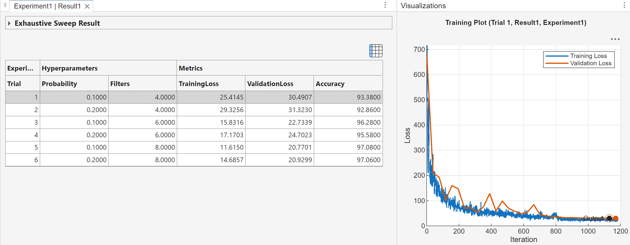
Run Experiment

When you run the experiment, Experiment Manager trains the network defined by the setup function six times. Each trial uses a different combination of hyperparameter values.

This experiment creates a training plot for each trial which you can use to visualize the progress while the experiment is running. To display the training plot, select a trial in the table of results, and on the Review Results section of the toolstrip, click Training Plot.

The table also displays the accuracy of the trial, as determined by the custom metric function Accuracy. You can show or hide columns by clicking the button above the table.

By default, Experiment Manager runs one trial at a time. For information about running multiple trials at the same time or offloading your experiment as a batch job in a cluster, see Run Experiments in Parallel and Offload Experiments as Batch Jobs to a Cluster.

Evaluate Results

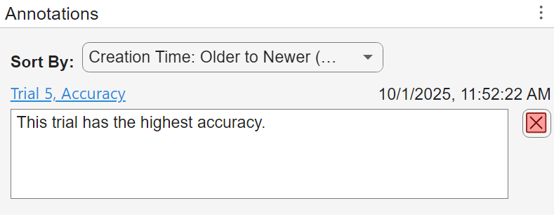
To find the best result for your experiment, sort the table of results by accuracy. In the table of results, point to the header of the Accuracy variable, click the sort icon, and select the Sort in Descending Order. The trial with the highest accuracy appears at the top of the results table. You can record that this trial has the highest accuracy in an annotation. Right-click the first trial in the sorted table, click Add Annotation, and then type your observation.

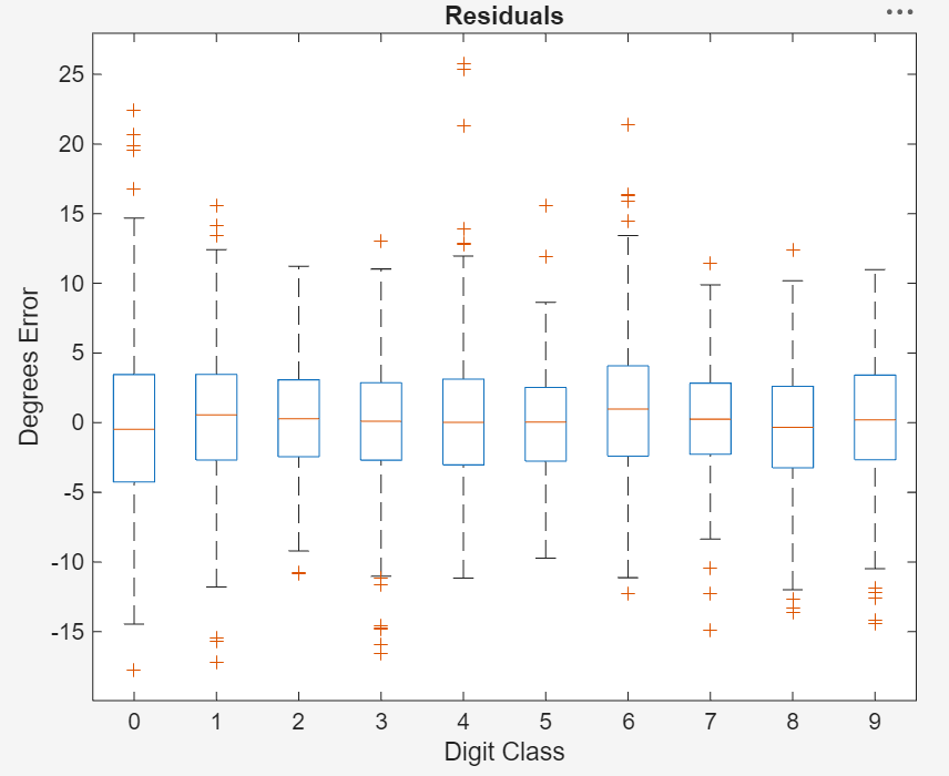
To test the performance of an individual trial, export the trained network and display a box plot of the residuals for each digit class.

1. Select the trial with the highest accuracy.

2. On the toolstrip, click Export > Trained Network.

3. In the dialog window, enter the name of a workspace variable for the exported network.

4. Define a function that creates a residual box plot for each digit. The digit classes with highest accuracy have a mean close to zero and little variance. Use reshape to group the residuals by digit class.

function plotResiduals(net)
[XValidation,~,YValidation] = digitTest4DArrayData;
YPredicted = predict(net,XValidation);
predictionError = YValidation - YPredicted;
residualMatrix = reshape(predictionError,500,10);
figure
boxplot(residualMatrix,...
    "Labels",["0","1","2","3","4","5","6","7","8","9"])
xlabel("Digit Class")
ylabel("Degrees Error")
title("Residuals")
end

5. In the Command Window, use the exported network as the input to the plotResiduals function.

plotResiduals(trainedNetwork)