Lateral Control Tutorial
This example shows how to control the steering angle of a vehicle that is following a planned path while changing lanes, using the Lateral Controller Stanley block.
Overview
Vehicle control is the final step in a navigation system and is typically accomplished using two independent controllers:
Lateral Controller: Adjust the steering angle such that the vehicle follows the reference path. The controller minimizes the distance between the current vehicle position and the reference path.
Longitudinal Controller: While following the reference path, maintain the desired speed by controlling the throttle and the brake. The controller minimizes the difference between the heading angle of the vehicle and the orientation of the reference path.
This example focuses on lateral control in the context of path following in a constant longitudinal velocity scenario. In the example, you will:
Learn about the algorithm behind the Lateral Controller Stanley block.
Create a driving scenario using the Driving Scenario Designer app and generate a reference path for the vehicle to follow.
Test the lateral controller in the scenario using a closed-loop Simulink® model.
Visualize the scenario and the associated simulation results using the Bird's-Eye Scope.
Lateral Controller
The Stanley lateral controller [1] uses a nonlinear control law to minimize the cross-track error and the heading angle of the front wheel relative to the reference path. The Lateral Controller Stanley block computes the steering angle command that adjusts a vehicle's current pose to match a reference pose.

Depending on the vehicle model used in deriving the control law, the Lateral Controller Stanley block has two configurations [1]:
Kinematic bicycle model: The kinematic model assumes that the vehicle has negligible inertia. This configuration is mainly suitable for low-speed environments, where inertial effects are minimal. The steering command is computed based on the reference pose, the current pose, and the velocity of the vehicle.
Dynamic bicycle model: The dynamic model includes inertia effects: tire slip and steering servo actuation. This more complicated, but more accurate, model allows the controller to handle realistic dynamics. In this configuration, the controller also requires the path curvature, the current yaw rate of the vehicle, and the current steering angle to compute the steering command.
You can set the configuration through the Vehicle model parameter in the block dialog box.
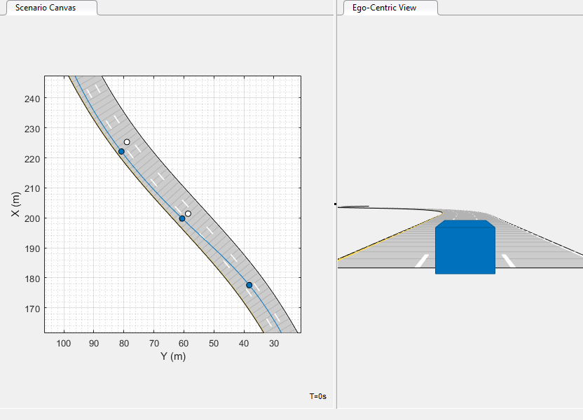
Scenario Creation
The scenario was created using the Driving Scenario Designer app. This scenario includes a single, three-lane road and the ego vehicle. For detailed steps on adding roads, lanes, and vehicles, see Create Driving Scenario Interactively and Generate Synthetic Sensor Data. In this scenario, the vehicle:
Starts in the middle lane.
Switches to the left lane after entering the curved part of the road.
Changes back to the middle lane.
Throughout the simulation, the vehicle runs at a constant velocity of 10 meters/second. This scenario was exported from the app as a MATLAB® function using the Export > Export MATLAB Function button. The exported function is named helperCreateDrivingScenario.m. The roads and actors from this scenario were saved to the scenario file LateralControl.mat.
Model Setup
Open the Simulink tutorial model.
open_system('LateralControlTutorial')

The model contains the following main components:
A Lateral Controller Variant Subsystem (Simulink) which contains two Lateral Controller Stanley blocks, one configured with a kinematic bicycle model and the other one with a dynamic bicycle model. They both can control the steering angle of the vehicle. You can specify the active one from the command line. For example, to select the Lateral Controller Stanley Kinematic block, use the following command:
variant = 'LateralControlTutorial/Lateral Controller';
set_param(variant, 'LabelModeActivechoice', 'Kinematic');
A
HelperPathAnalyzer.mblock, which provides the reference signal for the lateral controller. Given the current pose of the vehicle, it determines the reference pose by searching for the closest point to the vehicle on the reference path.A Vehicle and Environment subsystem, which models the motion of the vehicle using a Vehicle Body 3DOF (Vehicle Dynamics Blockset) block. The subsystem also models the environment by using a Scenario Reader block to read the roads and actors from the LateralControl.mat scenario file.
Opening the model also runs the helperLateralControlTutorialSetup.m script, which initializes data used by the model. The script loads certain constants needed by the Simulink model, such as vehicle parameters, controller parameters, the road scenario, and reference poses. In particular, the script calls the previously exported function helperCreateDrivingScenario.m to build the scenario. The script also sets up the buses required for the model by calling helperCreateLaneSensorBuses.m.
You can plot the road and the planned path using:
helperPlotRoadAndPath(scenario, refPoses)

Simulate Scenario
When simulating the model, you can open the Bird's-Eye Scope to analyze the simulation. After opening the scope, click Find Signals to set up the signals. Then run the simulation to display the vehicle, the road boundaries, and the lane markings. The image below shows the Bird's-Eye Scope for this example at 25 seconds. At this instant, the vehicle has switched to the left lane.

You can run the full simulation and explore the results using the following command:
sim('LateralControlTutorial');
You can also use the Simulink® Scope (Simulink) in the Vehicle and Environment subsystem to inspect the performance of the controller as the vehicle follows the planned path. The scope shows the maximum deviation from the path is less than 0.3 meters and the largest steering angle magnitude is less than 3 degrees.
scope = 'LateralControlTutorial/Vehicle and Environment/Scope';
open_system(scope)

To reduce the lateral deviation and oscillation in the steering command, use the Lateral Controller Stanley Dynamic block and simulate the model again:
set_param(variant, 'LabelModeActivechoice', 'Dynamic');
sim('LateralControlTutorial');

Conclusions
This example showed how to simulate lateral control of a vehicle in a lane changing scenario using Simulink. Compared with the Lateral Controller Stanley Kinematic block, the Lateral Controller Stanley Dynamic block provides improved performance in path following with smaller lateral deviation from the reference path.
References
[1] Hoffmann, Gabriel M., Claire J. Tomlin, Michael Montemerlo, and Sebastian Thrun. "Autonomous Automobile Trajectory Tracking for Off-Road Driving: Controller Design, Experimental Validation and Racing." American Control Conference. 2007, pp. 2296-2301.
Supporting Functions
helperPlotRoadAndPath Plot the road and the reference path
function helperPlotRoadAndPath(scenario,refPoses)
%helperPlotRoadAndPath Plot the road and the reference path
h = figure('Color','white');
ax1 = axes(h, 'Box','on');
plot(scenario,'Parent',ax1)
hold on
plot(ax1,refPoses(:,1),refPoses(:,2),'b')
xlim([150, 300])
ylim([0 150])
ax1.Title = text(0.5,0.5,'Road and Reference Path');
end
See Also
Apps
Blocks
- Lateral Controller Stanley | Lane Keeping Assist System (Model Predictive Control Toolbox) | Vehicle Body 3DOF (Vehicle Dynamics Blockset)