Model a Refrigeration Cycle with Varying Conditions
R2026bThis example extends the Model a Refrigeration Cycle workflow. That workflow develops a refrigeration system that initializes and operates at a nominal operating state. In that example, you choose pressure and enthalpy operating points and load and environment conditions, build open-loop test harnesses, and then close the refrigeration loop.
This example extends the system to support varying heat loads, varying environmental temperatures, and startup from a soaked state. To enable dynamic operation, the example introduces controllers, refrigerant storage volumes, and initialization techniques.
Mechanical Design
Engineering Requirements
The system represents an electric-vehicle battery cooling system. A vapor-compression refrigeration cycle cools a battery coolant loop through an evaporator.
Nominal battery heat: 3 kW
Maximum heat load capacity: 12 kW
COP: 2.6
Compressor work: 1.1 kW
Coolant temperature: 22 degC
Ambient: 20 degC
Refrigerant: R-1234yf
Coolant: 50/50 Ethylene-Glycol
A PI controller for an electronic expansion valve (EEV) maintains superheat at the evaporator outlet.
Nominal Operation:
Evaporating temperature: 5 degC
Evaporator superheat: 4.85 degC
Evaporator pressure drop: 5 kPa
Condensing temperature: 60 degC
Condenser subcooling: 9.2 degC
Condenser pressure drop: 10 kPa
Compressor isentropic efficiency: 70%
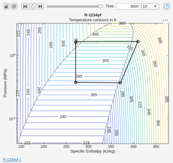
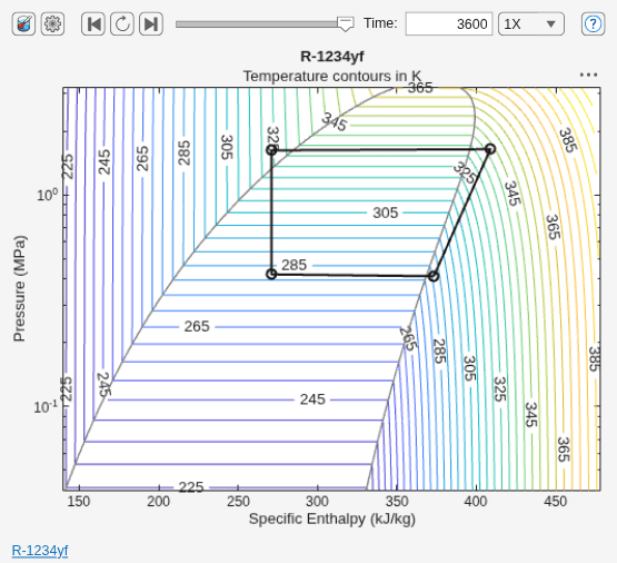
The four p-h state points of the nominal refrigeration cycle are:
Location | Point Number | Pressure (p) | Specific Enthalpy (h) |
Evaporator outlet | 1 | 0.368 MPa | 371.0 kJ/kg |
Condenser inlet | 2 | 1.652 MPa | 409.7 kJ/kg |
Condenser outlet | 3 | 1.642 MPa | 270.9 kJ/kg |
Evaporator inlet | 4 | 0.373 MPa | 270.9 kJ/kg |
Open-Loop Model for Nominal Conditions
Follow the Model a Refrigeration Cycle tutorial to create two open-loop harness models.
An evaporator/compressor harness.
A condenser/expansion-valve harness.
To view the harness model created by this workflow, open ModelADynamicRefrigerationCycleNominalOpenLoop.
open_system('ModelADynamicRefrigerationCycleNominalOpenLoop');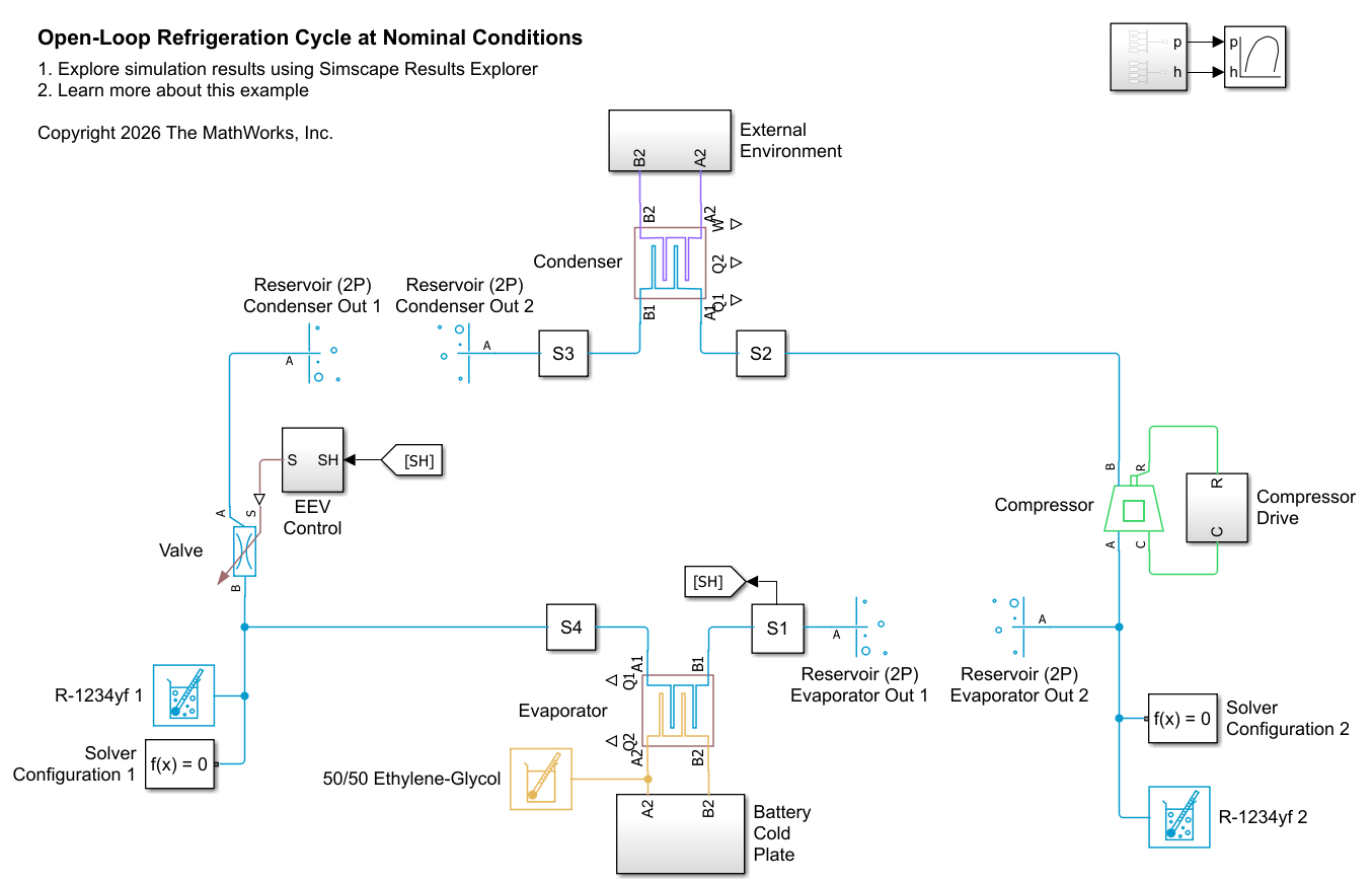
The ModelADynamicRefrigerationCycleNominalOpenLoop model combines the two refrigeration-system harnesses into a single model. Each harness uses Reservoir (2P) blocks to impose identical boundary conditions on the refrigeration components.
The harnesses are modeled as separate Simscape networks to emphasize that they represent two independent refrigeration subsystems. As a result, each harness requires its own Solver Configuration block and R‑1234yf fluid property block. Alternatively, you could connect the harnesses through an Infinite Flow Resistance (2P) block and use a single shared Solver Configuration block and R‑1234yf fluid property block.
The reservoir boundary conditions of the independent harness models make it easier to verify operating points and diagnose component-level issues before closing the loop.
Key Modeling Choices
Electronic Expansion Valve
Open the EEV Control subsystem.
open_system('ModelADynamicRefrigerationCycleNominalOpenLoop/EEV Control');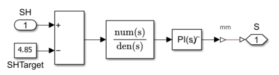
The electronic expansion valve (EEV) uses a PI controller that adjusts the valve opening to maintain 4.85 degC of superheat at the evaporator outlet. The superheat target is representative of a typical automotive refrigeration system. Decreasing valve opening decreases the refrigerant flow rate, while increasing the opening increases the flow rate. These changes affect the evaporator pressure and saturation temperature, which in turn affect the evaporator operating temperature. The chosen controller gains and time constants provide stable and responsive control over the operating conditions considered in this example. Under nominal operating conditions, the EEV provides system stability.
The valve is sized so that full travel (20 mm) corresponds to a maximum mass flow rate of 0.12 kg/s. At the nominal operating point, the valve opening is 5 mm and the mass flow rate is 0.03 kg/s. This sizing supports a maximum heat load capacity of 12 kW.
Compressor Drive
Open the Compressor Drive subsystem.
open_system('ModelADynamicRefrigerationCycleNominalOpenLoop/Compressor Drive');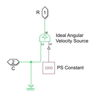
The Compressor Drive subsystem maintains the nominal compressor speed of 1000 rpm.
External Environment
Open the External Environment subsystem.
open_system('ModelADynamicRefrigerationCycleNominalOpenLoop/External Environment');
The External Environment subsystem represents airflow through the condenser. A Flow Rate Source sucks air from an inlet reservoir, through the condenser connected at ports A2 and B2, and into an outlet reservoir.
Battery Cold Plate
Open the Battery Cold Plate subsystem.
open_system('ModelADynamicRefrigerationCycleNominalOpenLoop/Battery Cold Plate');
The Battery Cold Plate subsystem represents the heat load on the evaporator. A Flow Rate Source drives the coolant through the evaporator connected at ports A2 and B2. The evaporator decreases the temperature of the coolant.
Simulate the open-loop model and confirm that the cycle reaches the four target operating points on the p-h diagram.
sim('ModelADynamicRefrigerationCycleNominalOpenLoop');
open_system('ModelADynamicRefrigerationCycleNominalOpenLoop/P-H Diagram (2P)');
Closed-Loop Model for Nominal Conditions
After validating the open-loop harness models, close the loop. Remove all four reservoirs and connect the harnesses together. Delete one Solver Configuration block and one R-1234yf property block because now there is only one two-phase network.
open_system('ModelADynamicRefrigerationCycleNominalClosedLoop');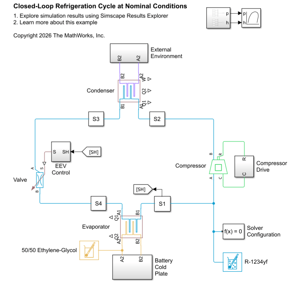
Simulate the closed-loop model and observe the p-h diagram.
open_system('ModelADynamicRefrigerationCycleNominalClosedLoop/P-H Diagram (2P)');
sim('ModelADynamicRefrigerationCycleNominalClosedLoop');
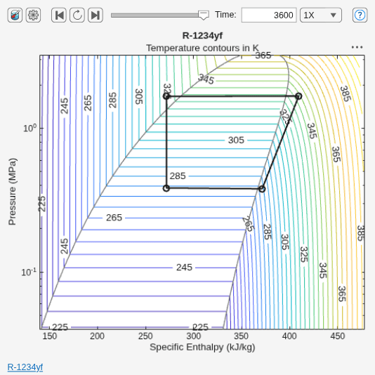
The complete refrigeration cycle reaches the nominal operating point. Small rounding differences between the open-loop and closed-loop operating points occur when the closed-loop model initial conditions differ slightly from the nominal design.
Modify the Model for Transient Behavior
The nominal closed-loop model operates correctly for a constant heat load and constant ambient condition. However, real refrigeration systems rarely operate under steady conditions. As operating conditions change, temperatures, pressures, and flow rates throughout the refrigeration cycle also change. Dynamic operation therefore requires control systems that adapt to changing conditions and fluid storage volumes that accommodate transient changes in refrigerant and coolant mass distributions.
This section describes modifications to the ModelADynamicRefrigerationCycleNominalClosedLoop model so that it can respond to changing heat loads, changing ambient temperatures, and startup transients.
Open the model that has been modified for transient behavior, ModelADynamicRefrigerationCycleVaryingClosedLoop:
open_system('ModelADynamicRefrigerationCycleVaryingClosedLoop');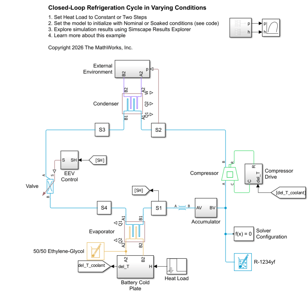
Model Modifications
To simulate varying heat loads and environmental conditions, the modified model has two added capabilities in each fluid network:
Flow rate control adjusts heat transfer rates in the heat exchangers.
Buffering volume in the fluid loop absorbs pressure and state transients when conditions change. In a dynamic system, fluid mass must be stored somewhere when flow rates and heat transfer rates temporarily become unbalanced during transitions between steady operating points. Buffering volumes provide temporary fluid storage and prevent large pressure and state transients.
Refrigerant Loop
Open the Compressor Drive subsystem.
open_system('ModelADynamicRefrigerationCycleVaryingClosedLoop/Compressor Drive');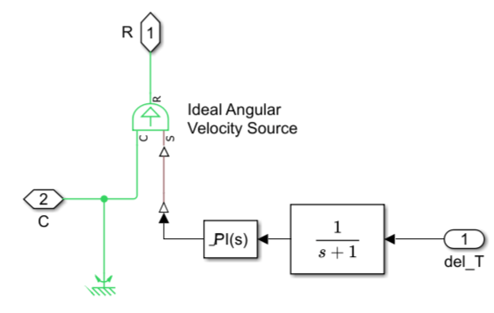
A PI controller for compressor speed adjusts the refrigerant flow rate to try to maintain the coolant at 22 degC at the cold plate outlet. Under varying loads, the refrigerant mass flow must adjust to match the changing cooling demand. A 1-second time lag represents realistic actuator dynamics and enables stable closed-loop behavior without introducing excessive control lag.
Open the Accumulator subsystem.
open_system('ModelADynamicRefrigerationCycleVaryingClosedLoop/Accumulator');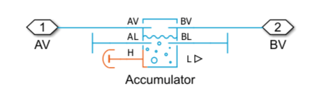
The refrigerant loop now has an accumulator at the evaporator outlet. During transients, refrigerant can accumulate in or leave the evaporator faster than the compressor and expansion valve can respond. The accumulator provides additional refrigerant storage that accommodates these flow imbalances and helps stabilize the system. An Accumulator Receiver (2P) block also separates liquid from vapor. This phase separation ensures that only vapor leaves through the top port BV, helping prevent liquid refrigerant from reaching the compressor during transients in this model. Other refrigeration systems may instead use a receiver at the condenser outlet to provide refrigerant storage and ensure that liquid flows to the expansion valve.
Coolant Loop
Open the Battery Cold Plate subsystem.
open_system('ModelADynamicRefrigerationCycleVaryingClosedLoop/Battery Cold Plate');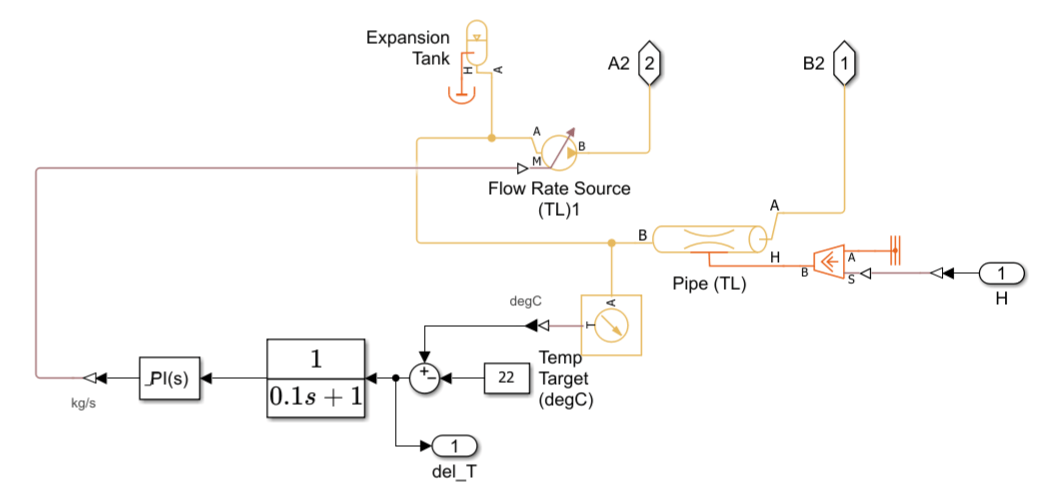
In place of the original Reservoir (TL) blocks, this subsystem uses a Pipe (TL) block that can dynamically respond to the heat load applied at thermal port H and the fluid cooled by the evaporator. The Pipe (TL) block represents the coolant flow path through a battery cooling plate. The pipe dimensions correspond to approximately 5 m of coolant flow channel, which is representative of a vehicle battery cooling system designed for a nominal heat load of 3 kW.
A PI controller adjusts the pump flow rate to try to maintain 22 degC at the Pipe (TL) outlet. The coolant outlet temperature target of 22 degC represents a battery thermal management system operating near its desired temperature range. The controller gains and time constants provide stable and responsive temperature regulation over the operating conditions considered in this example.
An expansion tank with a compressible air pocket accommodates coolant density changes and helps prevent large pressure fluctuations in the coolant loop.
Moist Air Network
Open the External Environment subsystem.
open_system('ModelADynamicRefrigerationCycleVaryingClosedLoop/External Environment');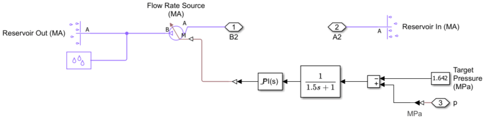
A PI controller for condenser fan speed adjusts the airflow to maintain the target refrigerant condensing pressure. The fan-speed control allows the condenser capacity to adapt as ambient temperature or refrigerant heat load changes.
Heat Load
Open the Heat Load subsystem.
open_system('ModelADynamicRefrigerationCycleVaryingClosedLoop/Heat Load', 'force');
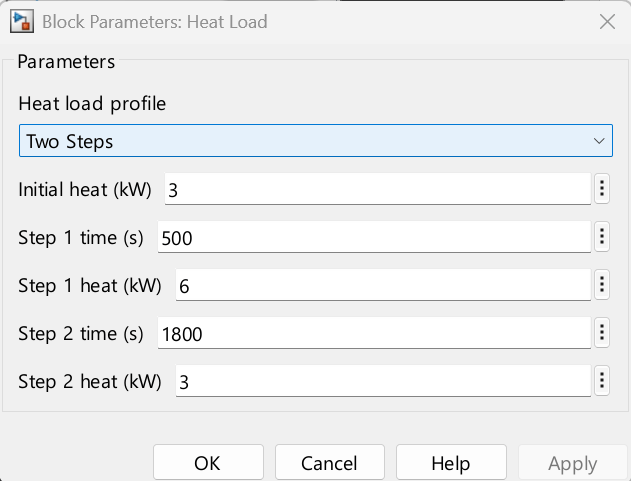
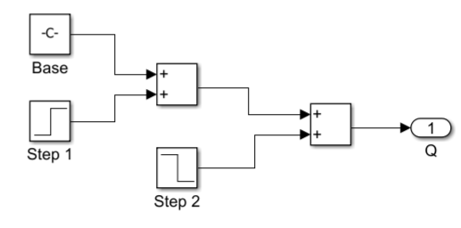
Simulink blocks set the heat flow rate that controls a Controlled Heat Flow Rate Source block that connects to the Pipe (TL) thermal port H. Here, the heat load is modeled as two steps during the simulation.
Simulate and confirm that the model simulates under the transient conditions:
sim('ModelADynamicRefrigerationCycleVaryingClosedLoop');
open_system('ModelADynamicRefrigerationCycleVaryingClosedLoop/P-H Diagram (2P)');
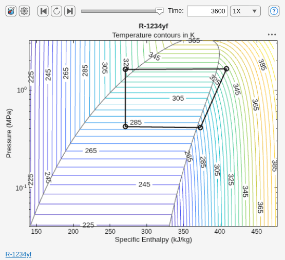
Initialize from a Soaked State
A soaked system has been off long enough for all components to reach the ambient temperature. Correct initialization requires setting fluid states to the ambient temperature while preserving the amount of refrigerant and coolant contained in the system during nominal operation. Otherwise, the system starts with the wrong amount of fluid and cannot reach the nominal operating point after startup.
The following process computes initial values for the soaked state:
Determine the refrigerant mass and volume at the nominal operating point.
Determine the refrigerant pressure and energy state at the ambient temperature and update the corresponding initial targets in the model.
Determine pressure in the coolant loop at the ambient temperature and update the corresponding initial targets in the model.
Update the initial values of the moist air components.
Update the initial controller outputs.
Step 1 - Compute the Refrigeration Charge Density
The soaked-state refrigerant pressure depends on both temperature and the amount of refrigerant contained in the system. The refrigerant charge density (mass per volume) is a constant property in a refrigeration loop when the volume is constant and mass cannot enter or leave the system. Therefore, the first step is to determine the refrigerant charge at the nominal operating point.
Compute the total refrigeration loop volume, mass, and density at the nominal operating point. This model contains three blocks that hold refrigerant volume: the evaporator, accumulator, and condenser.
Obtain the volume of the components from their volume parameters and the fluid mass from the simlog. The ModelADynamicRefrigerationCycleCalculateRefrigerantMassVolume script obtains these quantities and calculates the charge density.
ModelADynamicRefrigerationCycleCalculateRefrigerantMassVolume;
disp(TableMassVolume);
                   Volume (l)    Mass (kg)
                   __________    _________

    Evaporator        0.15       0.0049919
    Accumulator        0.5        0.011109
    Condenser          0.5           0.194
    Total             1.15         0.21011
The average charge density in the refrigeration loop is:
disp(value(chargeDensity, 'kg/m^3'));182.7009
Step 2 - Compute the Refrigerant States at the Soaked Temperature
When a refrigeration system is off, pressure equalizes throughout the loop as the temperature reaches the atmospheric temperature. The soaked-state pressure is therefore determined by the refrigerant charge and ambient temperature, rather than by the normal operating-point pressures.
The refrigerantChargeProperties function calculates fluid states based on the charge density and temperature.
[pressureSoaked, hSoaked, ~, uNormSoaked] = refrigerantChargeProperties( ...
    'ModelADynamicRefrigerationCycleVaryingClosedLoop/R-1234yf', chargeDensity, simscape.Value(Tatm, 'degC'));
The ModelADynamicRefrigerationCycleInitSoaked2P script applies the computed pressure, enthalpy, and internal energy to the evaporator, accumulator, and condenser in the ModelADynamicRefrigerationCycleVaryingClosedLoop model.
ModelADynamicRefrigerationCycleInitSoaked2P;
The script sets the accumulator to a saturated mixture (VLE) initial state and derives the initial liquid mass fraction from the normalized internal energy:
RefrigerantAccumulatorInitialLiquidMassFraction = 1 - value(uNormSoaked, '1');
Step 3 - Compute the Coolant States at the Soaked Temperature
Coolant mass in the thermal liquid loop must also be conserved. To determine the coolant pressure at the ambient temperature, this example uses a simplified harness model that starts from the nominal operating point and cools to the ambient temperature. If the expansion tank is sufficiently large relative to the coolant volume, coolant pressure remains nearly constant regardless of temperature. In that case, you can model a constant soaked pressure instead of simulating the coolant harness.
Open the coolant harness model.
open_system('ModelADynamicRefrigerationCycleCoolantLoopHarness');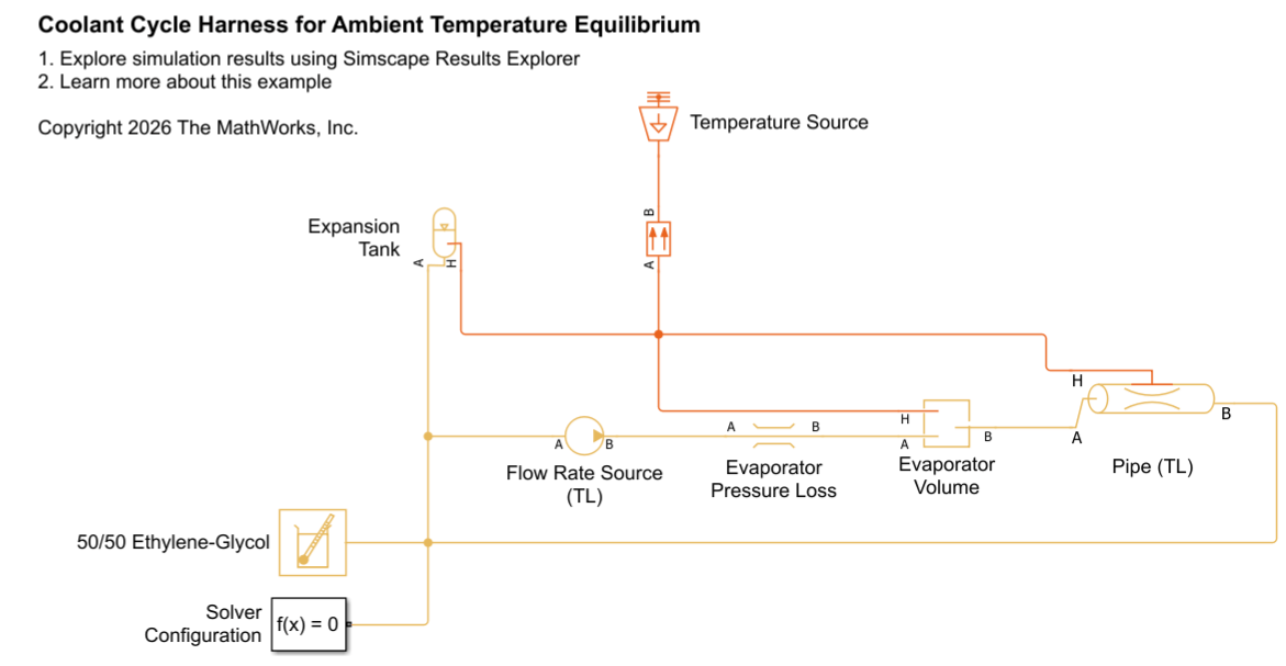
The harness is currently configured to represent the coolant mass and pressure losses. A Constant Volume Chamber (TL) block and a Flow Resistance (TL) block represent the Evaporator. The mass flow rate is set to 0 kg/s. A Temperature Source block set to the ambient temperature connects to the thermal ports of all blocks containing coolant volume. After the coolant reaches the ambient temperature, the pressure in the harness provides the soaked-state coolant pressure that can be used to initialize the full refrigeration model.
A similar approach could be used for the refrigerant loop. However, the refrigerantChargeProperties function provides a simpler way to determine soaked-state refrigerant conditions. The coolant loop is more difficult to treat analytically because the fluid volume changes with the state of the expansion tank.
Simulate the model and obtain the coolant pressure from the last time step in the simlog.
sim(ModelADynamicRefrigerationCycleCoolantLoopHarness);
CoolantPressure = simlog_ModelADynamicRefrigerationCycleCoolantLoopHarness.Pipe_TL.p_I.series.values('MPa');
CoolantPressureSoaked = CoolantPressure(end);
The ModelADynamicRefrigerationCycleInitSoakedTL script applies initial conditions to the coolant loop blocks in the full refrigeration model, ModelADynamicRefrigerationCycleVaryingClosedLoop.
ModelADynamicRefrigerationCycleInitSoakedTL;
Step 4 - Update Initial Values of the Moist Air Components for the Soaked State
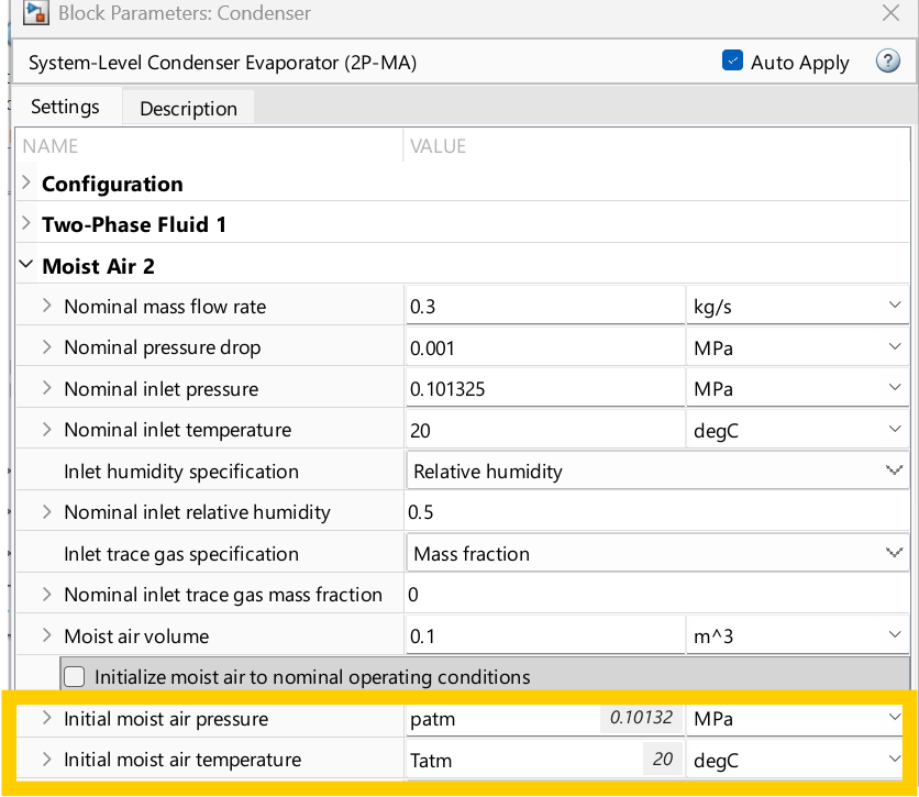
During a soaked condition, air in the condenser is in equilibrium with the surrounding environment. Initializing the moist air side to nominal operating conditions would create an artificial temperature and pressure difference at startup. Uncheck the Initialize moist air to nominal operating conditions parameter in the Condenser block. The parameters in the Condenser block are already configured so that unchecking the option will initialize the Moist Air side of the condenser at atmospheric pressure and temperature.
In the ModelADynamicRefrigerationCycleVaryingClosedLoop model, the Moist Air Reservoirs already have atmospheric conditions, so they do not require any changes for the soaked initialization.
set_param('ModelADynamicRefrigerationCycleVaryingClosedLoop/Condenser', 'nominal_init_MA', 'false')
Step 5 - Update Initial Values of the Controllers for the Soaked State
The ModelADynamicRefrigerationCycleInitSoakedControllers script sets the PI controller integrators to small nonzero initial values. The controllers do not initialize at their nominal operating values because the system starts far from the nominal operating state. The nonzero values provide an initial control action during startup and help prevent the controllers from becoming stuck at zero output. Real systems often use dedicated startup control logic, but this example uses fixed initial controller values to simplify the initialization procedure and controller output saturation.
ModelADynamicRefrigerationCycleInitSoakedControllers;
Simulate Starting from a Soaked State at 20 degC
Simulate from the soaked state. The system starts up and reaches the nominal operating points:
sim('ModelADynamicRefrigerationCycleVaryingClosedLoop');
open_system('ModelADynamicRefrigerationCycleVaryingClosedLoop/P-H Diagram (2P)');
Simulate Starting from a Soaked State at 50 degC
Next, start up the system on a hotter day with an ambient temperature of 50 degC. The refrigerant and coolant mass in the system remain the same, but the equilibrium fluid states change with ambient temperature.
Recalculate the initial states in the refrigerant and coolant loops for the hotter ambient temperature.
Tatm = 50; % [degC]

[pressureSoaked, hSoaked, ~, uNormSoaked] = refrigerantChargeProperties( ...
    'ModelADynamicRefrigerationCycleVaryingClosedLoop/R-1234yf', chargeDensity, simscape.Value(Tatm, 'degC'));
ModelADynamicRefrigerationCycleInitSoaked2P;

sim(ModelADynamicRefrigerationCycleCoolantLoopHarness);
CoolantPressure = simlog_ModelADynamicRefrigerationCycleCoolantLoopHarness.Pipe_TL.p_I.series.values('MPa');
CoolantPressureSoaked = CoolantPressure(end);
ModelADynamicRefrigerationCycleInitSoakedTL;
Simulate the model.
sim('ModelADynamicRefrigerationCycleVaryingClosedLoop');
open_system('ModelADynamicRefrigerationCycleVaryingClosedLoop/P-H Diagram (2P)');
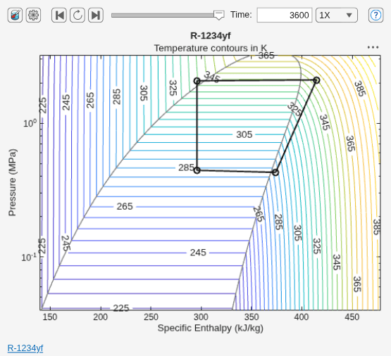
The p-h diagram shows operating points at slightly higher pressures, reflecting the hotter ambient conditions.
To return to initializing the system at nominal operation, run the ModelADynamicRefrigerationCycleNominalInit script to configure block parameters:
ModelADynamicRefrigerationCycleNominalInit;
Key Takeaways
Validate nominal operation using open-loop harness models.
Add controllers and storage volumes to handle varying operating conditions.
Initialize fluid states and controller outputs for the soaked state initialization.
Preserve refrigerant and coolant mass during soaked-state initialization.

