Find Vegetation in a Multispectral Image

Step 1: Import Color-Infrared Channels from a Multispectral Image File

This example finds vegetation in a LANDSAT Thematic Mapper image covering part of Paris, France, made available courtesy of Space Imaging, LLC. Seven spectral channels (bands) are stored in one file in the Erdas LAN format. The LAN file, paris.lan, contains a 7-channel 512-by-512 Landsat image. A 128-byte header is followed by the pixel values, which are band interleaved by line (BIL) in order of increasing band number. Pixel values are stored as unsigned 8-bit integers, in little-endian byte order.

The first step is to read bands 4, 3, and 2 from the LAN file using the MATLAB® function multibandread.

Channels 4, 3, and 2 cover the near infrared (NIR), the visible red, and the visible green parts of the electromagnetic spectrum. When they are mapped to the red, green, and blue planes, respectively, of an RGB image, the result is a standard color-infrared (CIR) composite. The final input argument to multibandread specifies which bands to read, and in which order, so that you can construct a composite in a single step.

CIR = multibandread('paris.lan',[512, 512, 7],'uint8=>uint8',...
                    128,'bil','ieee-le',{'Band','Direct',[4 3 2]});

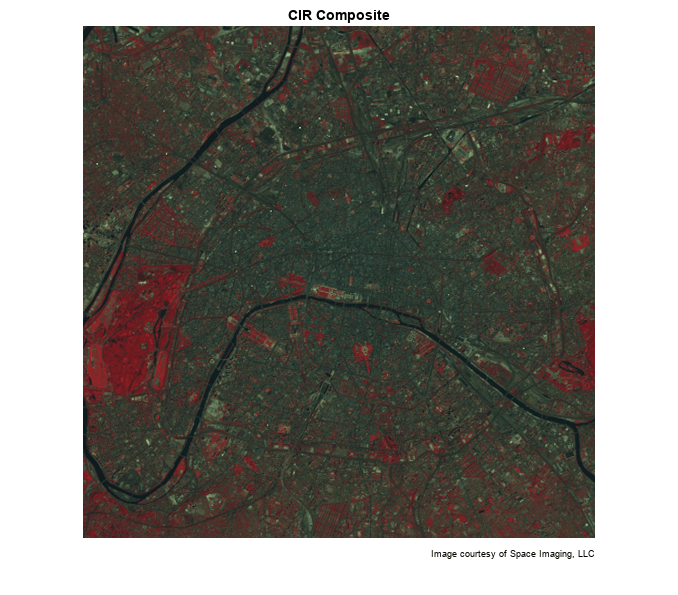
Variable CIR is a 512-by-512-by-3 array of class uint8. It is an RGB image, but with false colors. When the image is displayed, red pixel values signify the NIR channel, green values signify the visible red channel, and blue values signify the visible green channel.

In the CIR image, water features are very dark (the Seine River) and green vegetation appears red (parks and shade trees). Much of the image appearance is due to the fact that healthy, chlorophyll-rich vegetation has a high reflectance in the near infrared. Because the NIR channel is mapped to the red channel in the composite image, any area with a high vegetation density appears red in the display. A noticeable example is the area of bright red on the left edge, a large park (the Bois de Boulogne) located west of central Paris within a bend of the Seine River.

imshow(CIR)
title('CIR Composite')
text(size(CIR,2),size(CIR,1) + 15,...
  'Image courtesy of Space Imaging, LLC',...
  'FontSize',7,'HorizontalAlignment','right')

By analyzing differences between the NIR and red channels, you can quantify this contrast in spectral content between vegetated areas and other surfaces such as pavement, bare soil, buildings, or water.

Step 2: Construct an NIR-Red Spectral Scatter Plot

A scatter plot is a natural place to start when comparing the NIR channel (displayed as red pixel values) with the visible red channel (displayed as green pixel values). It's convenient to extract these channels from the original CIR composite into individual variables. It's also helpful to convert from class uint8 to class single so that the same variables can be used in the NDVI computation below, as well as in the scatter plot.

NIR = im2single(CIR(:,:,1));
R = im2single(CIR(:,:,2));

Viewing the two channels together as grayscale images, you can see how different they look.

imshow(R)
title('Visible Red Band')

imshow(NIR)
title('Near Infrared Band')

With one simple call to the plot command in MATLAB, you can create a scatter plot displaying one point per pixel (as a blue cross, in this case), with its x-coordinate determined by its value in the red channel and its y-coordinate by the value its value in the NIR channel.

plot(R,NIR,'+b')
ax = gca;
ax.XLim  = [0 1];
ax.XTick = 0:0.2:1;
ax.YLim  =  [0 1];
ax.YTick = 0:0.2:1;
axis square
xlabel('red level')
ylabel('NIR level')
title('NIR vs. Red Scatter Plot')

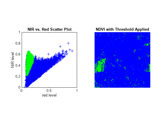
The appearance of the scatter plot of the Paris scene is characteristic of a temperate urban area with trees in summer foliage. There's a set of pixels near the diagonal for which the NIR and red values are nearly equal. This "gray edge" includes features such as road surfaces and many rooftops. Above and to the left is another set of pixels for which the NIR value is often well above the red value. This zone encompasses essentially all of the green vegetation.

Step 3: Compute Vegetation Index via MATLAB® Array Arithmetic

Observe from the scatter plot that taking the ratio of the NIR level to red level would be one way to locate pixels containing dense vegetation. However, the result would be noisy for dark pixels with small values in both channels. Also notice that the difference between the NIR and red channels should be larger for greater chlorophyll density. The Normalized Difference Vegetation Index (NDVI) is motivated by this second observation. It takes the (NIR - red) difference and normalizes it to help balance out the effects of uneven illumination such as the shadows of clouds or hills. In other words, on a pixel-by-pixel basis subtract the value of the red channel from the value of the NIR channel and divide by their sum.

ndvi = (NIR - R) ./ (NIR + R);

Notice how the array-arithmetic operators in MATLAB make it possible to compute an entire NDVI image in one simple command. Recall that variables R and NIR have class single. This choice uses less storage than class double but unlike an integer class also allows the resulting ratio to assume a smooth gradation of values.

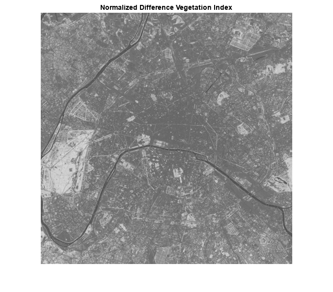
Variable ndvi is a 2-D array of class single with a theoretical maximum range of [-1 1]. You can specify these theoretical limits when displaying ndvi as a grayscale image.

figure
imshow(ndvi,'DisplayRange',[-1 1])
title('Normalized Difference Vegetation Index')

The Seine River appears very dark in the NDVI image. The large light area near the left edge of the image is the park (Bois de Boulogne) noted earlier.

Step 4: Locate Vegetation -- Threshold the NDVI Image

In order to identify pixels most likely to contain significant vegetation, apply a simple threshold to the NDVI image.

threshold = 0.4;
q = (ndvi > threshold);

The percentage of pixels selected is thus

100 * numel(NIR(q(:))) / numel(NIR)

ans = 
5.2204

or about 5 percent.

The park and other smaller areas of vegetation appear white by default when displaying the logical (binary) image q.

imshow(q)
title('NDVI with Threshold Applied')

Step 5: Link Spectral and Spatial Content

To link the spectral and spatial content, you can locate above-threshold pixels on the NIR-red scatter plot, re-drawing the scatter plot with the above-threshold pixels in a contrasting color (green) and then re-displaying the threshold NDVI image using the same blue-green color scheme. As expected, the pixels having an NDVI value above the threshold appear to the upper left of the rest and correspond to the redder pixels in the CIR composite displays.

Create the scatter plot, then display the thresholded NDVI.

figure
subplot(1,2,1)
plot(R,NIR,'+b')
hold on
plot(R(q(:)),NIR(q(:)),'g+')
axis square
xlabel('red level')
ylabel('NIR level')
title('NIR vs. Red Scatter Plot')

subplot(1,2,2)
imshow(q)
colormap([0 0 1; 0 1 0]);
title('NDVI with Threshold Applied')