Automatic Differentiation Background

What Is Automatic Differentiation?

Automatic differentiation (also known as autodiff, AD, or algorithmic differentiation) is a set of techniques for numerically evaluating derivatives (such as gradients and Jacobians) of a mathematical function. The method uses symbolic rules for differentiation, which are more accurate than finite difference approximations. Unlike a purely symbolic approach that performs large symbolic computations, automatic differentiation numerically evaluates expressions early in the computations. In other words, automatic differentiation evaluates derivatives at particular numeric values; it does not construct symbolic expressions for derivatives.

• Forward mode automatic differentiation evaluates a numerical derivative of a mathematical function by performing elementary derivative operations concurrently with the operations of evaluating the function itself. As detailed in the next section, MATLAB^® performs these operations on a computational graph.

• Reverse mode automatic differentiation uses an extension of the forward mode computational graph to enable the computation of a gradient by a reverse traversal of the graph. While computing the mathematical function and its derivative, MATLAB records operations in a data structure called a trace.

As many researchers have noted (for example, Baydin, Pearlmutter, Radul, and Siskind [1]), for a scalar function of many variables, reverse mode calculates the gradient more efficiently than forward mode. For further background, see [2].

In MATLAB, you can specify to use automatic differentiation as the calculation method for some derivatives. For example, for an ode object that represents a system of equations, you can set its JacobianMethod property to "autodiff" to calculate the Jacobians using automatic differentiation.

Forward Mode

Consider the problem of evaluating this function and its gradient:

$$f(x)=x_1\exp \left(-\frac{1}{2}\left(x_1^2+x_2^2\right)\right).$$

Automatic differentiation works at particular points. For this example, let x₁ = 2 and x₂ = 1/2.

This computational graph encodes the calculation of the function f(x).

To compute the gradient of f(x) using forward mode, you follow the same graph in the same direction but modify the computation based on the elementary rules of differentiation. To further simplify the calculation, you fill in the value of the derivative of each subexpression u_i as you go. To compute the entire gradient, you must traverse the graph twice, once for the partial derivative with respect to each independent variable. Each subexpression in the chain rule has a numeric value, so the entire expression has the same sort of computational graph as the function itself.

The computation is a repeated application of the chain rule. In this example, the derivative of f with respect to x₁ expands to this expression:

$$\begin{array}{c}\frac{df}{d{x}_1}=\frac{d{u}_6}{d{x}_1}\\ =\frac{\partial u_6}{\partial u_{-1}}+\frac{\partial u_6}{\partial u_5}\frac{\partial u_5}{\partial x_1}\\ =\frac{\partial u_6}{\partial u_{-1}}+\frac{\partial u_6}{\partial u_5}\frac{\partial u_5}{\partial u_4}\frac{\partial u_4}{\partial x_1}\\ =\frac{\partial u_6}{\partial u_{-1}}+\frac{\partial u_6}{\partial u_5}\frac{\partial u_5}{\partial u_4}\frac{\partial u_4}{\partial u_3}\frac{\partial u_3}{\partial x_1}\\ =\frac{\partial u_6}{\partial u_{-1}}+\frac{\partial u_6}{\partial u_5}\frac{\partial u_5}{\partial u_4}\frac{\partial u_4}{\partial u_3}\frac{\partial u_3}{\partial u_1}\frac{\partial u_1}{\partial x_1}.\end{array}$$

Let $${\dot{u}}_i$$ represent the derivative of the expression u_i with respect to x₁. Using the evaluated values of u_i from the function evaluation, you compute the partial derivative of f with respect to x₁ as shown in the following figure. Notice that all the values of $${\dot{u}}_i$$ become available as you traverse the graph from top to bottom.

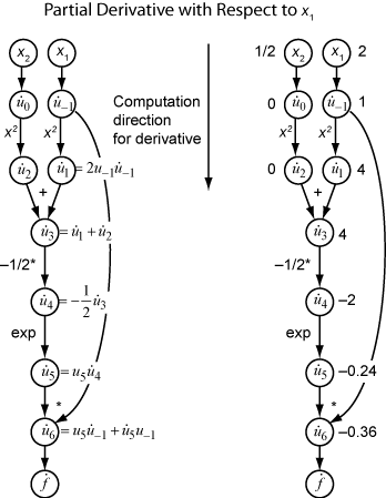
To compute the partial derivative with respect to x₂, you traverse a similar computational graph. Therefore, when you compute the gradient of the function, the number of graph traversals is the same as the number of variables. This process can be slow for many applications, when the objective function or nonlinear constraints depend on many variables.

Reverse Mode

Reverse mode uses one forward traversal of a computational graph to set up the trace. Then it computes the entire gradient of the function in one traversal of the graph in the opposite direction. For problems with many variables, this mode is far more efficient.

The theory behind reverse mode is also based on the chain rule, along with associated adjoint variables denoted with an overbar. The adjoint variable for u_i is

$${\overline{u}}_i=\frac{\partial f}{\partial u_i}.$$

In terms of the computational graph, each outgoing arrow from a variable contributes to the corresponding adjoint variable by its term in the chain rule. For example, the variable u_–1 has outgoing arrows to two variables, u₁ and u₆. The graph has the associated equation

$$\begin{array}{c}\frac{\partial f}{\partial u_{-1}}=\frac{\partial f}{\partial u_1}\frac{\partial u_1}{\partial u_{-1}}+\frac{\partial f}{\partial u_6}\frac{\partial u_6}{\partial u_{-1}}\\ ={\overline{u}}_1\frac{\partial u_1}{\partial u_{-1}}+{\overline{u}}_6\frac{\partial u_6}{\partial u_{-1}}.\end{array}$$

In this calculation, recalling that $$u_1=u_{-1}^2$$ and u₆ = u₅u_–1, you obtain

$${\overline{u}}_{-1}={\overline{u}}_{1}2u_{-1}+{\overline{u}}_6{u}_5.$$

During the forward traversal of the graph, MATLAB calculates the intermediate variables u_i. During the reverse traversal, starting from the seed value $${\overline{u}}_6=\frac{\partial f}{\partial f}=1$$, the reverse mode computation obtains the adjoint values for all variables. Therefore, reverse mode computes the gradient in just one pass, requiring much less time compared to forward mode.

The following computational graph shows how to compute the gradient in reverse mode for the function

$$f(x)=x_1\exp \left(-\frac{1}{2}\left(x_1^2+x_2^2\right)\right).$$

Again, let x₁ = 2 and x₂ = 1/2. The reverse mode computation relies on the u_i values that are obtained during the forward traversal of the original computational graph. On the right side of the figure, the computed values of the adjoint variables appear next to the adjoint variable names, using the formulas from the left side of the figure.

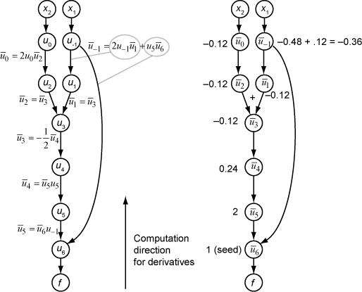
The final gradient values appear as $${\overline{u}}_0=\frac{\partial f}{\partial u_0}=\frac{\partial f}{\partial x_2}$$ and $${\overline{u}}_{-1}=\frac{\partial f}{\partial u_{-1}}=\frac{\partial f}{\partial x_1}$$.

References

[1] Baydin, Atilim Gunes, Barak A. Pearlmutter, Alexey Andreyevich Radul, and Jeffrey Mark Siskind. "Automatic Differentiation in Machine Learning: A Survey." Journal of Machine Learning Research 18, no. 153 (2018): 1–43. https://arxiv.org/abs/1502.05767.

[2] "Automatic differentiation." Wikipedia, October 31, 2025. https://en.wikipedia.org/wiki/Automatic_differentiation.