optimizeDesign
R2026bSyntax
Description
Examples
Define the performance specifications of a second-order DSM.
outputTable=table(); outputTable.Test=["ACMeas";"ACMeas";"ACMeas";"ACMeas";"ACMeas"]; outputTable.Name={'SNR';'SFDR';'SINAD';'ENOB';'NoiseFloor'}; outputTable.Units={'dB';'dB';'dB';'bits';'dB'}; outputTable.Spec={'> 72';'> 74';'> 72';'maximize 11.5';'< -78'}
outputTable = 5×4 table
Test Name Units Spec
________ ______________ ________ _________________
"ACMeas" {'SNR' } {'dB' } {'> 72' }
"ACMeas" {'SFDR' } {'dB' } {'> 74' }
"ACMeas" {'SINAD' } {'dB' } {'> 72' }
"ACMeas" {'ENOB' } {'bits'} {'maximize 11.5'}
"ACMeas" {'NoiseFloor'} {'dB' } {'< -78' }
Define the variables to optimize.
variableTable=table();
variableTable.parameters={'a1';'a2';'b1';'b2'};
variableTable.values=["0.15:0.005:0.16";"0.55:0.005:0.7";"0.15:0.005:0.16";"0.55:0.005:0.7"]variableTable = 4×2 table
parameters values
__________ _________________
{'a1'} "0.15:0.005:0.16"
{'a2'} "0.55:0.005:0.7"
{'b1'} "0.15:0.005:0.16"
{'b2'} "0.55:0.005:0.7"
Create the msbOptimizer object.
moptimizer = msbOptimizer(SimulationEnvironment='simulink',OutputsSetup=outputTable,VariableSetup=variableTable,DesignName='DSM2ndOrder')
moptimizer =
msbOptimizer with properties:
DesignName: 'DSM2ndOrder'
Solver: "surrogateopt"
SimulationEnvironment: 'simulink'
BestSolution: []
BestMetrics: []
FinalOptimizerStatus: []
OutputsSetup: [5×4 table]
ParametersSetup: [4×2 table]
ParameterNames: ["a1" "a2" "b1" "b2"]
ParameterValues: ["0.15:0.005:0.16" "0.55:0.005:0.7" "0.15:0.005:0.16" "0.55:0.005:0.7"]
Eflag: []
Trials: []
Constraints: [5×9 table]
Corners: []
Optimize the parameters.
[sol,metric] = moptimizer.optimizeDesign
Maximum number of simulations: 100 Number of parallel simulations: 1
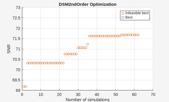
Optimizer was able to meet all the specifications.
sol = 4×2 table
Name Value
____ _____
"a1" 0.15
"a2" 0.575
"b1" 0.155
"b2" 0.635
metric = 5×4 table
Name FinalMetrics Specs Units
____________ ____________ _______________ ______
"SNR" 72.519 "> 72" "dB"
"SFDR" 80.869 "> 74" "dB"
"SINAD" 72.519 "> 72" "dB"
"ENOB" 11.754 "maximize 11.5" "bits"
"NoiseFloor" -80.755 "< -78" "dB"
As you can see, the function meets the required specifications. You can use the check point file to continue further optimization from the current state.
Input Arguments
Circuit design to optimize, specified as an msbOptimizer object.
The object includes the name of the simulation environment, the name of the circuit
design, the performance specifications, and the variables to optimize.
Name-Value Arguments
Specify optional pairs of arguments as
Name1=Value1,...,NameN=ValueN, where Name is
the argument name and Value is the corresponding value.
Name-value arguments must appear after other arguments, but the order of the
pairs does not matter.
Example: [sol,metric] = obj.optimizeDesign(ProgressPlot='true')
optimizes the circuit design defined in the obj object and shows the
optimization progress in a plot.
Number of parallel simulations per iteration, specified as a nonnegative integer scalar.
Data Types: double
Maximum number of simulations to run, specified as a nonnegative integer scalar.
The default is max(100,10*nvar), where nvar is the number of problem
variables.
Data Types: double
Minimum number of random sample points to create at the start of the optimization
phase, specified as a nonnegative integer scalar. The default is max(20,2*nvar), where nvar is the number of problem variables.
For more information, see Surrogate Optimization Algorithm (Global Optimization Toolbox).
Note
The function ignores this argument if the Solver is set
to essabopt.
Data Types: double
Show optimization progress in a plot.
Data Types: logical
Metric name to plot on the progress plot, specified as a string or character vector. The default is the first metric on the constraint table.
Name of the file to create checkpoints and restart the optimization process, specified as a string or character vector.
Use the checkpoint file for optimization. The function can use this argument only after the creation of a checkpoint file at the end of a simulation run.
If the Solver is set to surrogateopt, the
checkpoint file saves the internal surrogate solver data.
If the Solver is set to essabopt, the
checkpoint file saves the entire population, performance history, and optimizer
state.
Data Types: logical
Optimization solver used to optimize circuit parameters. You can choose between
surrogateopt and essabopt.
Note
To use the essabopt optimization technique, you need a
license for Deep Learning Toolbox™.
Handle to a custom objective function that runs simulation and returns the objective and constraint violations, specified as an object handle.
You can use this argument to support non-standard simulation workflows such as running Simulink® simulations or extracting custom metrics from the logged signals. For more information, see Custom Objective Functions for Simulink Simulation.
Initial points for surrogate optimization, specified as a matrix or structure.
When you set Solver to essabopt, the
function ignores this argument. The function rather sets the internal population by max(20,5*nvar).
Data Types: double
Random number generator seed, specified as a nonnegative integer scalar.
Data Types: double
Random number generator algorithm used by optimization solver, specified as a string.
Data Types: char
Output Arguments
Optimized variables or parameters, returned as a table. The elements of the table
match the variables or parameters defined in the VariableSetup
argument in msbOptimizer object.
Performance metrics using optimized variables or parameters, returned as a table.
The elements of the table match the variables or parameters defined in the
OutputsSetup argument in msbOptimizer
object.
More About
To run non-standard Simulink simulations, you can use the ObjectiveFunction argument
to create custom objective functions. The custom function must accept parameter indices as a
matrix of variable values.
| Argument Name | Argument Type | Description |
|---|---|---|
x | Input | Matrix of variable indices, specified as integers. The elements are mapped to
variablevalues. |
variableNames | Input | String array of parameter names. |
contraintTable | Input | Internal constraint table derived from
OutputsSetup. |
model | Input | Name of the Simulink model. |
variableValues | Input | Cell array of value vectors, one per parameter. |
out.Fval | Output | Scalar objective per design. A negative value means the function meets all constraints. |
out.Ineq | Output | Constraint violations. |
You can use this template to create your custom objective function:
% Custom Objective Function Template function out = myCustomObjFcn(x, variableNames, constraintTable, model, variableValues) out.Fval = NaN(size(x,1), 1); out.Ineq = NaN(size(x,1), height(constraintTable)); for ii = 1:size(x,1) % Map indices to physical values for jj = 1:numel(variableNames) paramValue = variableValues{jj}(x(ii,jj)); % ... assign parameter, run simulation, extract metrics ... end end % Helper computes objective + constraint violations from results [out.Fval, out.Ineq] = msblks.optimization.surrogateOptHelper.getFvalIneq( ... size(x,1), resultsTable, constraintTable); end
objFcn = @(x) myCustomObjFcn(x, varNames, constrTable, modelName, varValues);
[sol, met] = optimizer.optimizeDesign('ObjectiveFunction', objFcn);The Efficient Surrogate Model-assisted Sizing Method for High-performance Analog Building Blocks (ESSAB) is a machine learning-based surrogate global optimization approach designed specifically for analog IC design. It combines differential evolution (DE) for design generation with an artificial neural network (ANN) for performance prediction. It uses a novel probability of further improvement (PFI) infill sampling criterion based on beta-distribution ranking.
ESSAB is designed for optimizing high-dimensional problems (more than 10 variables). But extremely high dimensions can degrade ANN prediction accuracy. Try to limit your design variables between 10 and 40.
Tips
Set
Solvertosurrogateoptfor general-purpose optimization problems with short simulation times or quick design verifications. This works best when the number of design variables is less than 10 or problems have discontinuous transitions.Set
Solvertoessaboptfor analog IC sizing problems with long simulation times or when accurate final design values are critical. It works best when the number of design variables is between 10 and 40 or problems have multiple constraints with stringent specifications.
Version History
Introduced in R2024b
MATLAB Command
You clicked a link that corresponds to this MATLAB command:
Run the command by entering it in the MATLAB Command Window. Web browsers do not support MATLAB commands.
Seleccione un país/idioma
Seleccione un país/idioma para obtener contenido traducido, si está disponible, y ver eventos y ofertas de productos y servicios locales. Según su ubicación geográfica, recomendamos que seleccione: .
También puede seleccionar uno de estos países/idiomas:
Cómo obtener el mejor rendimiento
Seleccione China (en idioma chino o inglés) para obtener el mejor rendimiento. Los sitios web de otros países no están optimizados para ser accedidos desde su ubicación geográfica.
América
- América Latina (Español)
- Canada (English)
- United States (English)
Europa
- Belgium (English)
- Denmark (English)
- Deutschland (Deutsch)
- España (Español)
- Finland (English)
- France (Français)
- Ireland (English)
- Italia (Italiano)
- Luxembourg (English)
- Netherlands (English)
- Norway (English)
- Österreich (Deutsch)
- Portugal (English)
- Sweden (English)
- Switzerland
- United Kingdom (English)