Minimize Energy of Piecewise Linear Mass-Spring System Using Cone Programming, Problem-Based
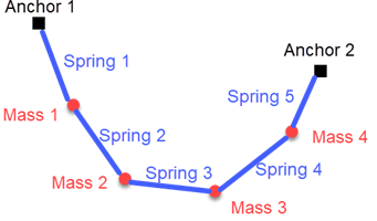
This example shows how to use the problem-based approach to find the equilibrium position of a mass-spring system hanging from two anchor points. The springs have piecewise linear tensile forces. The system consists of masses in two dimensions. Mass is connected to springs and . Springs and are also connected to separate anchor points. In this case, the zero-force length of spring is a positive length , and the spring generates force when stretched to length . The problem is to find the minimum potential energy configuration of the masses, where potential energy comes from the force of gravity and from stretching the nonlinear springs. The equilibrium occurs at the minimum energy configuration.
This illustration shows five springs and four masses suspended from two anchor points.
The potential energy of a mass at height is , where is the gravitational constant on Earth. Also, the potential energy of an ideal linear spring with the spring constant stretched to length is . In the current model, the spring is not ideal, but it has a nonzero resting length .
The mathematical basis of this example comes from Lobo, Vandenberghe, Boyd, and Lebret [1]. For a solver-based version of this example, see Minimize Energy of Piecewise Linear Mass-Spring System Using Cone Programming, Solver-Based.
Mathematical Formulation
The location of mass is , with the horizontal coordinate and vertical coordinate . Mass has potential energy due to gravity of . The potential energy in spring is , where is the length of the spring between mass and mass . Take anchor point 1 as the position of mass 0, and anchor point 2 as the position of mass . The preceding energy calculation shows that the potential energy of spring is
.
Reformulating this potential energy problem as a second-order cone programming problem requires the introduction of some new variables, as described in Lobo [1]. Create variables equal to the square root of the term .
Let be the unit column vector . Then . The problem becomes
(1)
Now consider as a free vector variable, not given by the previous equation for . Incorporate the relationship between and in the new set of cone constraints
(2)
The objective function is not yet linear in its variables, as required for coneprog. Introduce a new scalar variable . Notice that the inequality is equivalent to the inequality
. (3)
Now the problem is to minimize
(4)
subject to the cone constraints on and listed in (2) and the additional cone constraint (3). Cone constraint (3) ensures that . Therefore, problem (4) is equivalent to problem (1).
The objective function and cone constraints in problem (4) are suitable for solution with coneprog.
MATLAB® Formulation
Define six spring constants , six length constants , and five masses .
k = 40*(1:6);
l = [1 1/2 1 2 1 1/2];
m = [2 1 3 2 1];
g = 9.807;
Define optimization variables corresponding to the mathematical problem variables. For simplicity, set the anchor points as two virtual mass points x(1,:) and x(end,:). This formulation allows each spring to stretch between two masses.
nmass = length(m) + 2;
% k and l have nmass-1 elements
% m has nmass - 2 elements
x = optimvar("x",[nmass,2]);
t = optimvar("t",nmass-1,LowerBound=0);
y = optimvar("y",LowerBound=0);
Create an optimization problem and set the objective function to the expression in (4).
prob = optimproblem;
obj = dot(x(2:(end-1),2),m)*g + y;
prob.Objective = obj;
Create the cone constraints corresponding to expression (2).
conecons = optimineq(nmass - 1);
for ii = 1:(nmass-1)
    conecons(ii) = norm(x(ii+1,:) - x(ii,:)) - l(ii) <= sqrt(2/k(ii))*t(ii);
end
prob.Constraints.conecons = conecons;
Specify the anchor points anchor0 and anchorn. Create equality constraints specifying that the two virtual end masses are located at the anchor points.
anchor0 = [0 5];
anchorn = [5 4];
anchorcons = optimeq(2,2);
anchorcons(1,:) = x(1,:) == anchor0;
anchorcons(2,:) = x(end,:) == anchorn;
prob.Constraints.anchorcons = anchorcons;
Create the cone constraint corresponding to expression (3).
ycone = norm([2*t;(1-y)]) <= 1 + y;
prob.Constraints.ycone = ycone;
Solve Problem
The problem formulation is complete. Solve the problem by calling solve.
[sol,fval,eflag,output] = solve(prob);
Solving problem using coneprog.
Optimal solution found.
Plot the solution points and the anchors.
plot(sol.x(2:(nmass-1),1),sol.x(2:(nmass-1),2),"ro")
hold on
plot([sol.x(1,1),sol.x(end,1)],[sol.x(1,2),sol.x(end,2)],"ks")
plot(sol.x(:,1),sol.x(:,2),"b--")
legend("Calculated points","Anchor points","Springs",Location="best")
xlim([sol.x(1,1)-0.5,sol.x(end,1)+0.5])
ylim([min(sol.x(:,2))-0.5,max(sol.x(:,2))+0.5])
hold off
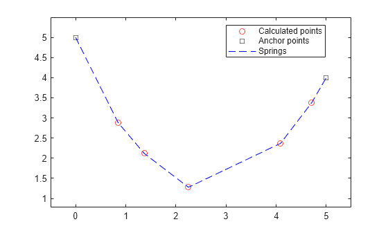
You can change the values of the parameters m, l, and k to see how they affect the solution. You can also change the number of masses; the code takes the number of masses from the data you supply.
References
[1] Lobo, Miguel Sousa, Lieven Vandenberghe, Stephen Boyd, and Hervé Lebret. “Applications of Second-Order Cone Programming.” Linear Algebra and Its Applications 284, no. 1–3 (November 1998): 193–228. https://doi.org/10.1016/S0024-3795(98)10032-0.