Backscatter Pedestrian
Libraries:
      Radar Toolbox
   
Description
The Backscatter Pedestrian block models the monostatic reflection of non-polarized electromagnetic signals from a walking pedestrian. The pedestrian walking model coordinates the motion of 16 body segments to simulate natural motion. The model also simulates the radar reflectivity of each body segment. From this model, you can obtain the position and velocity of each segment and the total backscattered radiation as the body moves.
Ports
Input
Incident radar signals on each body segment, specified as a complex-valued M-by-16 matrix. M is the number of samples in the signal. See Body Segment Indices for the column representing the incident signal at each body segment.
The size of the first dimension of the input matrix can vary to simulate a changing signal length. A size change can occur, for example, in the case of a pulse waveform with variable pulse repetition frequency.
Data Types: double
Complex Number Support: Yes
Incident signal directions on the body segments, specified as a real-valued
              2-by-16 matrix. Each column of ANG specifies the incident
              direction of the signal to the corresponding body part. Each column takes the form of
              an [AzimuthAngle;ElevationAngle] pair. Units are in degrees. See
                Body Segment Indices for the column
              representing the incident direction at each body segment.
Data Types: double
Heading of the pedestrian, specified as a scalar. Heading is measured in the xy-plane from the x-axis towards the y-axis. Units are in degrees.
Example: -34
Data Types: double
Output
Combined reflected radar signals, returned as a complex-valued
                M-by-1 column vector. M equals the same number
              of samples as in the input signal, X.
Data Types: double
Complex Number Support: Yes
Positions of body segments, returned as a real-valued 3-by-16 matrix. Each column
              represents the Cartesian position, [x;y;z], of one of 16 body
              segments. Units are in meters. See Body Segment Indices for the column
              representing the position of each body segment.
Data Types: double
Velocity of body segments, returned as a real-valued 3-by-16 matrix. Each column
              represents the Cartesian velocity, [vx;vy;vz], of one of 16 body
              segments. Units are in meters per second. See Body Segment Indices for the column
              representing the velocity of each body segment.
Data Types: double
Orientation axes of body segments, returned as a real-valued 3-by-3-by-16 array. Each page represents the 3-by-3 orientation axes of one of 16 body segments. Units are dimensionless. See Body Segment Indices for the page representing the orientation of each body segment.
Data Types: double
Parameters
Height of pedestrian, specified as a positive scalar. Units are in meters.
Data Types: double
Walking speed of the pedestrian, specified as a nonnegative scalar. The motion model limits the walking speed to 1.4 times the pedestrian height set in the Height (m) parameter. Units are in meters per second.
Data Types: double
Signal propagation speed, specified as a real-valued positive scalar. The default
            value of the speed of light is the value returned by
              physconst('LightSpeed').
Data Types: double
Carrier frequency of narrowband incident signals, specified as a positive scalar. Units are in Hz.
Example: 1e9
Data Types: double
Initial position of the pedestrian, specified as a 3-by-1 real-valued vector in the
            form of [x;y;z]. Units are in meters.
Data Types: double
Initial heading of the pedestrian, specified as a scalar. Heading is measured in the xy-plane from the x-axis towards y-axis. Units are in degrees.
Data Types: double
Block simulation, specified as Interpreted Execution or
              Code Generation. If you want your block to use the
              MATLAB® interpreter, choose Interpreted Execution. If
            you want your block to run as compiled code, choose Code
              Generation. Compiled code requires time to compile but usually runs
            faster.
Interpreted execution is useful when you are developing and tuning a model. The
            block runs the underlying System object™ in MATLAB. You can change and execute your model quickly. When you are satisfied
            with your results, you can then run the block using Code
              Generation. Long simulations run faster than in interpreted execution.
            You can run repeated executions without recompiling, but if you change any block
            parameters, then the block automatically recompiles before execution.
This table shows how the Simulate using parameter affects the overall simulation behavior.
When the Simulink® model is in Accelerator mode, the block mode specified
            using Simulate using overrides the simulation mode.
Acceleration Modes
| Block Simulation | Simulation Behavior | ||
| Normal | Accelerator | Rapid Accelerator | |
| Interpreted Execution | The block executes using the MATLAB interpreter. | The block executes using the MATLAB interpreter. | Creates a standalone executable from the model. | 
| Code Generation | The block is compiled. | All blocks in the model are compiled. | |
For more information, see Choosing a Simulation Mode (Simulink).
More About
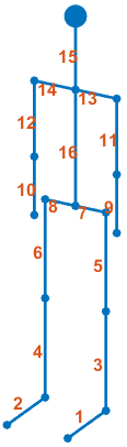
Body segment indices define which columns in the X, Ang, BPPOS, and BPVEL ports contain the data for a specific body segment. Body segment indices define which page in the Ax port contains the data for a specific body segments. For example, column 3 of X contains sample data for the left lower leg. Column 3 of Ang contains the arrival angle of the signal at the left lower leg.
| Body Segment | Index | |
|---|---|---|
| Left foot | 1 | 
 | 
| Right foot | 2 | |
| Left lower leg | 3 | |
| Right lower leg | 4 | |
| Left upper leg | 5 | |
| Right upper leg | 6 | |
| Left hip | 7 | |
| Right hip | 8 | |
| Left lower arm | 9 | |
| Right lower arm | 10 | |
| Left upper arm | 11 | |
| Right upper arm | 12 | |
| Left shoulder | 13 | |
| Right shoulder | 14 | |
| Head | 15 | |
| Torso | 16 | |
Extended Capabilities
C/C++ Code Generation
 Generate C and C++ code using Simulink® Coder™.
Version History
Introduced in R2021a
MATLAB Command
You clicked a link that corresponds to this MATLAB command:
Run the command by entering it in the MATLAB Command Window. Web browsers do not support MATLAB commands.
Seleccione un país/idioma
Seleccione un país/idioma para obtener contenido traducido, si está disponible, y ver eventos y ofertas de productos y servicios locales. Según su ubicación geográfica, recomendamos que seleccione: .
También puede seleccionar uno de estos países/idiomas:
Cómo obtener el mejor rendimiento
Seleccione China (en idioma chino o inglés) para obtener el mejor rendimiento. Los sitios web de otros países no están optimizados para ser accedidos desde su ubicación geográfica.
América
- América Latina (Español)
- Canada (English)
- United States (English)
Europa
- Belgium (English)
- Denmark (English)
- Deutschland (Deutsch)
- España (Español)
- Finland (English)
- France (Français)
- Ireland (English)
- Italia (Italiano)
- Luxembourg (English)
- Netherlands (English)
- Norway (English)
- Österreich (Deutsch)
- Portugal (English)
- Sweden (English)
- Switzerland
- United Kingdom (English)

